This is Biology
28 Nov 2021(中文版原文連結)
This September in Boston didn’t prolong the blazing heat of summer, but was full of the feeling of autumn. The wind kissed my face as I rode my bike down the bridge across the Charles River, making me feel like swimming in the cold water. The unusual cold September caused me to expect the early arrival of fall colors; however, the theory hike on the first weekend of October was not as colorful as I imagined. Unsurprisingly, theory and reality had a gap again!
I immediately started an exciting conversation about cross-disciplinary research between CS and Neuroscience with a new postdoc right after we started the hike on the White Dot trail of Mt. Monadnock. We talked a little bit about what problems we’ve been exploring respectively and then moved on to the difference between biology, CS, and Physics research. What kind of biology research is “closer to the reality”? How to justify a mathematical model being “biologically plausible”? During our intense debate, I suddenly saw the deep gulf (which is quite obvious, but I didn’t realize it before) between biologists and computer scientists: when talking about biological plausibility, the two parties are basically talking about totally different things!
As a CS-trained student, I understand that when we talk about biological plausibility, what we have in mind are “conditions” or “biological constraints” such as the local connectivity or the sparse activities of neurons. Then, the next step we usually do is using mathematical models to capture these conditions and start either abstract deductive analysis or computer simulation. However, for biologists, biological plausibility does not necessarily refer to a concrete checklist. It’s more like, after a huge amount of reading, experiments, and discussions, each of them gradually builds up their own intuition and worldview. As the experiments in biology contain so much noise and special cases, it’s nearly impossible to write down rigorous mathematical constraints and check them one by one objectively. So sometimes it’s actually quite interesting to see that biologists might not be as biologically plausible as computer scientists would imagine!
Cross-disciplinary research is challenging. Not only does one have to learn a lot of knowledge from other fields, but in my opinion, the most difficult part is to understand and appreciate the beauty in the other fields. I occasionally saw a book recommendation on Facebook for “This is Biology” by Ernst Mayr. Through this book, I finally got a chance to peek into the big picture of a great (evolutionary) biologist on biology.
A roller coaster ride of philosophy of biology
Originally, I had just thought to ask my roommate, an evolutionary biologist, to read and discuss This is Biology together. In the end, he enthusiastically invited friends from several different fields to form a reading group, and this began a roller coaster ride of building up my philosophy of biology.
The reason why I call this a roller coaster ride is that I was challenged and reshaped multiple times during these three months. Now that the ride has ended, I’m ready to bring my newly built values and beliefs to start my next journey. As there will be much more stimulus and growth in my future exploration in cross-disciplinary research, here I’m going to briefly take some notes on the enlightenments and changes This is Biology has brought to me.
The beauty and challenge in Biology
A physics friend used to joke with me that Biology is like collecting stamps, and its beauty is about the diversity and complexity in nature, while the job of biologists is to collect and record new discoveries. Relatively speaking, physics and math seem to delve deeper into the hidden symmetry and structure in nature and the abstract world. Implicitly, this shows some superiority of physics over biology. Indeed, physicists often have the confidence of having a deeper understanding of the world. In contrast, as biology is a relatively young field, many sub-fields are still in the stage of collecting more and more data and observations from experiments. But such a difference in their current development does not imply which field is easier and which is more difficult. At the frontier of a scientific field, as long as one keeps the curiosity to the unknown, the rigor of knowledge, and the persistence in quality, every step forward is incomparably important and irreplaceable.
I grew up in an environment with very little exposure to nature. Amidst the hustle and bustle of the city and the fantasy of the abstract (mathematical) world, I always had a hard time understanding and appreciating the beauty in biology. I still vividly remember the first time I talked about research with my roommate. When he told me he was going to spend a couple of years taking photos of butterfly specimens and writing programs to analyze the shape and color of their wings, I really didn’t understand why this counted as “doing research.” Why was he going to spend so much time on a single species out of millions? Why were six specimens for each type of butterfly sufficient? Why could they make any claim and result under seemingly weak correlations and evidence?
Indeed, from the perspectives of physics and math, biology may not be listed in the Hall of Fame for intellectual pursuit. But why do we compare biology with physics and math? Directly comparing these different disciplines is like comparing music and painting. Individuals’ preferences could influence rational thinking and discussion. In the end, the difference in “the sense of beauty” among different fields causes huge misunderstandings and even discriminations. So why not throw away our prejudices and try to revisit the beauty of biology?
From collecting stamps to playing jigsaw puzzle
Biodiversity is undoubtedly the main reason why people would think of biology as like collecting stamps. Currently, there are hundreds of sub-atomic atoms known in the world, but the number of butterfly species on Earth is nearly 20,000. If we think more carefully about how to classify organisms, we will notice that even properly defining what a species means is a highly non-trivial task. As biodiversity is so messy and dirty, where is its beautiful part? In some senses, biology indeed looks like collecting stamps since much work is spent on collecting, classifying, and processing data. So is this data collection process the beauty of biodiversity? To me, such a “collecting stamps” stage is just the first step of appreciating biodiversity. The real exciting part of biologists’ job is to figure out the underlying pattern and difference among the huge amount of noisy data.
Thus, in my opinion, the beauty of biology is more in the stage after collecting stamps. And I call it the “playing jigsaw puzzle” stage. At this stage, people need to put the messy data points (i.e., pieces of a jigsaw puzzle) with certain correlations together. Moreover, one should not be interfered by superficial similarities (e.g., in the jigsaw puzzle below, different orange pieces might come from different orange cats!). Even worse, most of the time, it is impossible to collect enough pieces, and hence biologists often have to figure out something insightful without seeing the whole picture.
As a comparison, physics and mathematics are more like playing board games or strategy games where one of the main challenges is to walk through a huge maze with a small number of local choices/rules and huge global possibilities.
So in order to build up a sense of beauty for appreciating biology, I think we should temporarily loosen our insistence of logical perfection (in the sense of having a theory from first principles) and focus more on how to get something useful and interesting out from the huge and messy experimental data. If one doesn’t appreciate such kinds of beauty, then it might also be hard to have a deeper appreciation in some of the modern developments/research in biology. But of course, I’m not here to ask every reader to change themselves and start to like biology after reading this article. I guess the point is more about discussing the intrinsic differences between biology and physics (also math and other natural sciences). In the end, I really hope people from different fields can have fewer misunderstandings and discriminations towards each other. And if they have more time, they can even learn a little about the challenges and hopes in other fields.
Anyway, as I started to appreciate more of the beauty of playing jigsaw puzzle in biology, I realized much more exciting and cute aspects to explore. Here, I would like to share three recent revelations I had: the beauty of diversity, the beauty of the individual, and the beauty of the experiment.
The beauty of diversity: I vividly recall when I first met my roommate, I truly didn't understand why he was so excited about seeing a new ant species (to be honest, I still haven't fully grasped it...). In retrospect, my previous pursuit of beauty was more about abstractions, forms, and symmetries, while the beauty of biodiversity is almost on the other side of the coin. Particularly, it's often about concrete objects, real practices, and special cases. Nevertheless, although the two senses of beauty are very different, they are not necessarily conflicting with each other. Each person would have a different inclination toward these two types of beauty due to their family and education. And it is totally fine for a person to stick to the beauty that they find more comfortable with. But after opening up their eyes to the other type of beauty, the whole world will start to look more colorful. In my case, after having more and more appreciation for the beauty of biodiversity, every flower and tree on the street began to tell their stories to me. I also got a wider range of feelings on the surroundings and knowledge, and sometimes they could even bring me inspirations and joys.
The beauty of individual: Every organism is a unique existence in the world, unlike every hydrogen atom that basically looks exactly the same in the experiment. While biologists are working on finding patterns within biodiversity, the discovery of patterns could also bring new understandings of an individual through their differences. By building up theories in biology, we not only aim to figure out the governing rules behind reality but also try to find our own new perspectives and angles to comprehend the subtle beauty of the individual.
The beauty of experiment: In physics, people verify theoretical models through extremely precise experiments. In contrast, experiments in biology often cannot achieve such precision, and hence people often have to make claims from limited data and resources. For example, in the butterfly research of my roommate, he uses only six individuals for each species (and he told me this is the highest standard). This is not because they don't want or they cannot use a hundred individuals for each species. It is simply infeasible for them to conduct such a huge experiment under limited time and hands. Such reality constraints (e.g., the number of data points, noise in the data, etc.) are like the logical rules in mathematics. Biologists really need to struggle among these constraints and design meaningful experiments. I would say this might not be much easier than a mathematician walking through the labyrinth of axioms.
Let me give two examples of decision-making experiments in neuroscience to help readers appreciate the beauty behind experimental design.
First, some background information: in the study of decision-making, neuroscientists aim to identify network structures that can be mapped to decision-making mechanisms. A major challenge is to rule out as many alternatives as possible so that experimental findings can only be explained by the proposed theoretical model. Therefore, in addition to designing devices, researchers must also design animal behavior tasks and interpretations of various possible outcomes.
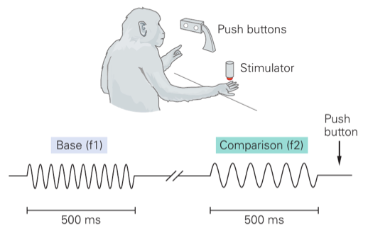
The first experiment is related to the somatosensory system. In this experiment, the fingers of a monkey are stimulated by a 20Hz stimulus for 500ms. Afterward, another stimulus with a different frequency is presented, and the monkey must decide whether the frequency of the second stimulus is higher or lower than that of the first stimulus.
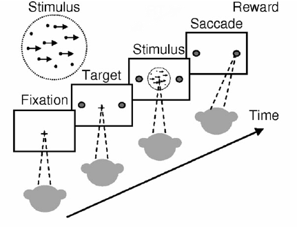
The second experiment is related to the visual system. In this experiment, a monkey first fixates on the central fixation spot of a screen (usually a cross) while dots are presented and move either from left to right or from right to left. Then, the monkey must decide whether the dots are moving toward the left or toward the right. Furthermore, a fraction of the dots move randomly to adjust the difficulty of the decision-making task.
Both of the above experiments are classic in the literature of decision-making. However, is one of them better than the other? If you think carefully, you will notice a big issue in the first experiment: there is a time gap between the two stimuli, and hence the monkey has to "memorize" the first vibration and compare it with the second one afterward. Note that this additional requirement of memorization (implicitly) increases the complexity of the task and hence makes it harder for the experimentalists to dissect the specific network that is responsible for the decision task only.
As for the second experiment, it first bypasses the memory issue by presenting all the information simultaneously. Second, it provides an adjustable parameter on the fraction of randomly moving dots to enable a more quantitative study of the underlying mechanism. Finally, the initial fixation is like a "reboot" that makes sure the monkey starts from a similar initial condition in every trial.
Different challenges: the lack of symmetry, emergence properties, objective meanings
To further establish a sense of beauty in biology, one has to embrace and understand its challenges. Here, I’d like to emphasize the following three challenges of biology from my personal view: the lack of symmetry, emergence properties, and the existence of objective meanings.
The lack of symmetry: It's not an exaggeration to say that the great success of modern physics is established on top of the brilliant observations of symmetry and asymmetry of the physical world. Symmetries not only lead to rich mathematics but also restrict the search space and enable abstract analysis (recommended reading: The Unreasonable Effectiveness of Mathematics in Physics). However, the jungle of biology seriously lacks those diverse and beautiful (and analyzable) symmetries. In my opinion, this is the root of the challenges to building good theories in biology. Thus, most of the mathematical or computational models in biology are more or less like a "description" as opposed to a "model" for the underlying reality.
Emergence properties: The so-called *emergence property* in biology is conceptually very similar to the *chaotic phenomenon* in physics: a bunch of applications of simple rules induces complicated results. Personally, I like to use a theoretical CS concept to think about emergence properties: one-wayness, i.e., easy to compute/manipulate in the forward direction, but hard to revert back to the initial starting point. How does an embryo develop into a mature organism? How are genes mapped to phenotypes? How do neurons' activities form computation, intelligence, and consciousness? Emergence properties make mechanical modeling and understanding extremely challenging. Either we get a rough statistical understanding via macroscopic analysis or get some models that soon become too complicated to understand as well (e.g., using deep learning to build a model). Meanwhile, the *reduction method* that is commonly used in physics also often oversimplifies the emergence properties and cannot capture multiple aspects simultaneously. Perhaps we really need a new methodology/framework to the traditional physical and mathematical methods?
Objective meanings: People always like to endow meanings to whatever we see. I still vividly remember during my last trip to Antelope Canyon, besides being amazed by the extraordinary workmanship of mother nature, I was also impressed by the creativity of the local tour guide. Within a few steps, you would hear something like "Look! This is the shark from Finding Nemo!" (see the figure below). I believe no one will believe that mother nature purposefully sculpted a shark in Antelope Canyon. However, this also reminds us to be aware of our own inductive bias while trying to understand nature. This reminds me of the comparison of *proximate cause* and *ultimate cause* mentioned in the book. It is truly subtle to be clear on what type of explanation one is talking about, especially when it is about correlations and causations. In a non-axiomatized discipline like biology, people unavoidably have to learn how to move forward without induction and/or deduction. Most of the time, the main scientific method is then based on abductive reasoning. In other words, all the knowledge is built on top of observations instead of logical axioms. Thus, there's even no so-called ground truth. There's only a better explanation rather than the best explanation. Nonetheless, "a better explanation" itself is very subjective, and the voice is often controlled by those experts in the field. Perhaps it is impossible to achieve a fully objective consensus in biology?
What are the knowledge, understanding, and theory in biology?
All the above examples and perspectives are serving for a key message Mayr wanted to convey from the very beginning of the book: there’s a need of different/new set of methodology and philosophy of science for biology (because those have been dominated by physics). I still remember that I always disagree with this opinion of Mayr and thought that he didn’t know enough physics. But now, even though I still don’t know if Mayr really knew some physics or not, I do know that my previous understanding of biology was too shallow.
So here I’d like to record the transition of my mindset and hope to prevent the non-biologists reader from discriminating biology. Meanwhile, this can also be an opportunity for biologists (like my roommate) to have more senses on the common prejudice from students with physics and math background.
Philosophy of science: the misunderstandings between biologists and physicists
I learned a little basic philosophy of science during my undergrad. It was nothing more than logical positivism, Kuhn’s paradigm shift, Popper’s falsification, etc. As ignorant as a kid, I had been regarding these as the axioms of doing science for a very long time. Not until I had much more independent thinking in the past few years did I realize the abundance of philosophy of science.
In the first paragraph of the Philosophy of Science section in the book, Mayr pointed out that even though there are several schools of thought, they all still center around physics (especially theoretical physics) and might not be that suitable for biology. I think this difference can be perfectly explained by the title of a famous paper by evolutionary biologist Stephen Jay Gould: “Evolution as Fact and Theory.” Notice that Gould didn’t say that evolution is reality or truth, while these two are exactly what most theoretical physicists are looking for! For example, this mindset can be seen from the title of the book by Nobel Prize in Physics laureate Roger Penrose: “The Road to Reality.”
Using more modern concepts to analyze the comparison of physics and biology, I would say the former is more like scientific realism while the latter is closer to instrumentalism. Simply speaking, scientific realism believes in the existence of an “ideal theory” and advocates that the goal of scientific research is to move closer and closer to the ideal theory. However, instrumentalism takes the opposite opinion and believes that scientific theories are tools for us to understand the world. Hence, the focus should be on explaining and predicting real-world phenomena.
Of course, I oversimplify the serious comparison and discussion on the different branches of philosophy of science. My main aim here is to plant some seeds in the readers’ minds so that you all can explore and build up your philosophy of science (The Stanford Encyclopedia of Philosophy could be a good starting point). As a friendly reminder, it is important to keep in mind that the philosophy of science ultimately is still just an assistant to help us clarify the goal and essence of scientific research. It’s not the end, and there’s no correct answer for it. Everyone can have different preferences, and the same person can even have different philosophical beliefs in different disciplines or sub-disciplines. If one can understand more perspectives, then this not only enriches your thinking, but also helps you think from other’s angles when talking to someone from a different field.
The role and possibility of math in biology?
As a theoretical computer scientist, an amateur mathematician, and a hobby physicist, I still have a strong pursuit (and need) for math and the beauty of abstraction. However, all the challenges in biology we have discussed above hardly do not make me wonder the possibility of applying math in biology. Recently, I came across this arXiv paper, “A mathematician’s view of the unreasonable ineffectiveness of mathematics in biology,” which gives a pretty good exposition of my concern. The author provides lots of observations and stories centering around the famous mathematician Israel Gelfand (who worked on biology after being well-established in pure math). I recommend it as a casual and enjoyable read.
My personal view is the following: Mathematics has been highly influenced by physics, and many branches correspond to a certain sub-discipline in physics. On the contrary, there are very few examples of new mathematics that were inspired by biology. This does not say that biology lacks mathematical potential. Maybe current mathematics is not yet ready for biology. We need someone to create new mathematics for biology!
But what kind of mathematics could be suitable for biology? Common mathematical tools used by bio-physicists or mathematical biologists are dynamical systems, differential equations, control theory, game theory, etc. In my opinion, there is a lack of an algorithmic lens. Here, what I meant by algorithms is something more general than the Turing machine sense. I meant something at the level of a software engineer, where there are huge programs with multiple sub-programs and their sub-sub-programs. Using such an algorithmic/software engineering view to understand biological systems can not only provide an analytic/logical methodology but also give different levels and granularities of understandings. The current development of computational biology could be something that is closest to what I have in mind. But most of the work there is still in the stage of writing models and running simulations. There is still no clean mathematical language that enables abstract analysis.
The reality of cross-disciplinary research, sympathy and understanding, next step
Besides the reading group for This is Biology, I also have been running a cross-disciplinary reading group (When neuroscience meets CS, math, and physics) with Brabeeba. These experiences make me fully understand that the challenges of cross-disciplinary interactions are bi-directional: besides learning more from the other fields and thinking in their shoes, the conversation should also start from the basis of the other person being interested in learning what you can bring. I then realized that to do cross-disciplinary research in the long-term, one should not only have solid foundations in different disciplines but also build up a sense of beauty and/or even get recognized by these fields to some extent. Quantitatively speaking, one should arrive at the basic graduate student level in the other field!
After realizing the challenges in front of my cross-disciplinary agenda did make me a bit frustrated in the beginning, but now I feel super excited and am very looking forward to what I will get to in all the different directions I’m interested in. I hope that I won’t forget the importance of sympathizing and understanding the distinctions of different fields and persistently push forward this lonely but fascinating journey.