$
\newcommand{\undefined}{}
\newcommand{\hfill}{}
\newcommand{\qedhere}{\square}
\newcommand{\qed}{\square}
\newcommand{\ensuremath}[1]{#1}
\newcommand{\bit}{\{0,1\}}
\newcommand{\Bit}{\{-1,1\}}
\newcommand{\Stab}{\mathbf{Stab}}
\newcommand{\NS}{\mathbf{NS}}
\newcommand{\ba}{\mathbf{a}}
\newcommand{\bc}{\mathbf{c}}
\newcommand{\bd}{\mathbf{d}}
\newcommand{\be}{\mathbf{e}}
\newcommand{\bh}{\mathbf{h}}
\newcommand{\br}{\mathbf{r}}
\newcommand{\bs}{\mathbf{s}}
\newcommand{\bx}{\mathbf{x}}
\newcommand{\by}{\mathbf{y}}
\newcommand{\bz}{\mathbf{z}}
\newcommand{\Var}{\mathbf{Var}}
\newcommand{\dist}{\text{dist}}
\newcommand{\norm}[1]{\\|#1\\|}
\newcommand{\etal}
\newcommand{\ie}
\newcommand{\eg}
\newcommand{\cf}
\newcommand{\rank}{\text{rank}}
\newcommand{\tr}{\text{tr}}
\newcommand{\mor}{\text{Mor}}
\newcommand{\hom}{\text{Hom}}
\newcommand{\id}{\text{id}}
\newcommand{\obj}{\text{obj}}
\newcommand{\pr}{\text{pr}}
\newcommand{\ker}{\text{ker}}
\newcommand{\coker}{\text{coker}}
\newcommand{\im}{\text{im}}
\newcommand{\vol}{\text{vol}}
\newcommand{\disc}{\text{disc}}
\newcommand{\bbA}{\mathbb A}
\newcommand{\bbB}{\mathbb B}
\newcommand{\bbC}{\mathbb C}
\newcommand{\bbD}{\mathbb D}
\newcommand{\bbE}{\mathbb E}
\newcommand{\bbF}{\mathbb F}
\newcommand{\bbG}{\mathbb G}
\newcommand{\bbH}{\mathbb H}
\newcommand{\bbI}{\mathbb I}
\newcommand{\bbJ}{\mathbb J}
\newcommand{\bbK}{\mathbb K}
\newcommand{\bbL}{\mathbb L}
\newcommand{\bbM}{\mathbb M}
\newcommand{\bbN}{\mathbb N}
\newcommand{\bbO}{\mathbb O}
\newcommand{\bbP}{\mathbb P}
\newcommand{\bbQ}{\mathbb Q}
\newcommand{\bbR}{\mathbb R}
\newcommand{\bbS}{\mathbb S}
\newcommand{\bbT}{\mathbb T}
\newcommand{\bbU}{\mathbb U}
\newcommand{\bbV}{\mathbb V}
\newcommand{\bbW}{\mathbb W}
\newcommand{\bbX}{\mathbb X}
\newcommand{\bbY}{\mathbb Y}
\newcommand{\bbZ}{\mathbb Z}
\newcommand{\sA}{\mathscr A}
\newcommand{\sB}{\mathscr B}
\newcommand{\sC}{\mathscr C}
\newcommand{\sD}{\mathscr D}
\newcommand{\sE}{\mathscr E}
\newcommand{\sF}{\mathscr F}
\newcommand{\sG}{\mathscr G}
\newcommand{\sH}{\mathscr H}
\newcommand{\sI}{\mathscr I}
\newcommand{\sJ}{\mathscr J}
\newcommand{\sK}{\mathscr K}
\newcommand{\sL}{\mathscr L}
\newcommand{\sM}{\mathscr M}
\newcommand{\sN}{\mathscr N}
\newcommand{\sO}{\mathscr O}
\newcommand{\sP}{\mathscr P}
\newcommand{\sQ}{\mathscr Q}
\newcommand{\sR}{\mathscr R}
\newcommand{\sS}{\mathscr S}
\newcommand{\sT}{\mathscr T}
\newcommand{\sU}{\mathscr U}
\newcommand{\sV}{\mathscr V}
\newcommand{\sW}{\mathscr W}
\newcommand{\sX}{\mathscr X}
\newcommand{\sY}{\mathscr Y}
\newcommand{\sZ}{\mathscr Z}
\newcommand{\sfA}{\mathsf A}
\newcommand{\sfB}{\mathsf B}
\newcommand{\sfC}{\mathsf C}
\newcommand{\sfD}{\mathsf D}
\newcommand{\sfE}{\mathsf E}
\newcommand{\sfF}{\mathsf F}
\newcommand{\sfG}{\mathsf G}
\newcommand{\sfH}{\mathsf H}
\newcommand{\sfI}{\mathsf I}
\newcommand{\sfJ}{\mathsf J}
\newcommand{\sfK}{\mathsf K}
\newcommand{\sfL}{\mathsf L}
\newcommand{\sfM}{\mathsf M}
\newcommand{\sfN}{\mathsf N}
\newcommand{\sfO}{\mathsf O}
\newcommand{\sfP}{\mathsf P}
\newcommand{\sfQ}{\mathsf Q}
\newcommand{\sfR}{\mathsf R}
\newcommand{\sfS}{\mathsf S}
\newcommand{\sfT}{\mathsf T}
\newcommand{\sfU}{\mathsf U}
\newcommand{\sfV}{\mathsf V}
\newcommand{\sfW}{\mathsf W}
\newcommand{\sfX}{\mathsf X}
\newcommand{\sfY}{\mathsf Y}
\newcommand{\sfZ}{\mathsf Z}
\newcommand{\cA}{\mathcal A}
\newcommand{\cB}{\mathcal B}
\newcommand{\cC}{\mathcal C}
\newcommand{\cD}{\mathcal D}
\newcommand{\cE}{\mathcal E}
\newcommand{\cF}{\mathcal F}
\newcommand{\cG}{\mathcal G}
\newcommand{\cH}{\mathcal H}
\newcommand{\cI}{\mathcal I}
\newcommand{\cJ}{\mathcal J}
\newcommand{\cK}{\mathcal K}
\newcommand{\cL}{\mathcal L}
\newcommand{\cM}{\mathcal M}
\newcommand{\cN}{\mathcal N}
\newcommand{\cO}{\mathcal O}
\newcommand{\cP}{\mathcal P}
\newcommand{\cQ}{\mathcal Q}
\newcommand{\cR}{\mathcal R}
\newcommand{\cS}{\mathcal S}
\newcommand{\cT}{\mathcal T}
\newcommand{\cU}{\mathcal U}
\newcommand{\cV}{\mathcal V}
\newcommand{\cW}{\mathcal W}
\newcommand{\cX}{\mathcal X}
\newcommand{\cY}{\mathcal Y}
\newcommand{\cZ}{\mathcal Z}
\newcommand{\bfA}{\mathbf A}
\newcommand{\bfB}{\mathbf B}
\newcommand{\bfC}{\mathbf C}
\newcommand{\bfD}{\mathbf D}
\newcommand{\bfE}{\mathbf E}
\newcommand{\bfF}{\mathbf F}
\newcommand{\bfG}{\mathbf G}
\newcommand{\bfH}{\mathbf H}
\newcommand{\bfI}{\mathbf I}
\newcommand{\bfJ}{\mathbf J}
\newcommand{\bfK}{\mathbf K}
\newcommand{\bfL}{\mathbf L}
\newcommand{\bfM}{\mathbf M}
\newcommand{\bfN}{\mathbf N}
\newcommand{\bfO}{\mathbf O}
\newcommand{\bfP}{\mathbf P}
\newcommand{\bfQ}{\mathbf Q}
\newcommand{\bfR}{\mathbf R}
\newcommand{\bfS}{\mathbf S}
\newcommand{\bfT}{\mathbf T}
\newcommand{\bfU}{\mathbf U}
\newcommand{\bfV}{\mathbf V}
\newcommand{\bfW}{\mathbf W}
\newcommand{\bfX}{\mathbf X}
\newcommand{\bfY}{\mathbf Y}
\newcommand{\bfZ}{\mathbf Z}
\newcommand{\rmA}{\mathrm A}
\newcommand{\rmB}{\mathrm B}
\newcommand{\rmC}{\mathrm C}
\newcommand{\rmD}{\mathrm D}
\newcommand{\rmE}{\mathrm E}
\newcommand{\rmF}{\mathrm F}
\newcommand{\rmG}{\mathrm G}
\newcommand{\rmH}{\mathrm H}
\newcommand{\rmI}{\mathrm I}
\newcommand{\rmJ}{\mathrm J}
\newcommand{\rmK}{\mathrm K}
\newcommand{\rmL}{\mathrm L}
\newcommand{\rmM}{\mathrm M}
\newcommand{\rmN}{\mathrm N}
\newcommand{\rmO}{\mathrm O}
\newcommand{\rmP}{\mathrm P}
\newcommand{\rmQ}{\mathrm Q}
\newcommand{\rmR}{\mathrm R}
\newcommand{\rmS}{\mathrm S}
\newcommand{\rmT}{\mathrm T}
\newcommand{\rmU}{\mathrm U}
\newcommand{\rmV}{\mathrm V}
\newcommand{\rmW}{\mathrm W}
\newcommand{\rmX}{\mathrm X}
\newcommand{\rmY}{\mathrm Y}
\newcommand{\rmZ}{\mathrm Z}
\newcommand{\bb}{\mathbf{b}}
\newcommand{\bv}{\mathbf{v}}
\newcommand{\bw}{\mathbf{w}}
\newcommand{\bx}{\mathbf{x}}
\newcommand{\by}{\mathbf{y}}
\newcommand{\bz}{\mathbf{z}}
\newcommand{\paren}[1]{( #1 )}
\newcommand{\Paren}[1]{\left( #1 \right)}
\newcommand{\bigparen}[1]{\bigl( #1 \bigr)}
\newcommand{\Bigparen}[1]{\Bigl( #1 \Bigr)}
\newcommand{\biggparen}[1]{\biggl( #1 \biggr)}
\newcommand{\Biggparen}[1]{\Biggl( #1 \Biggr)}
\newcommand{\abs}[1]{\lvert #1 \rvert}
\newcommand{\Abs}[1]{\left\lvert #1 \right\rvert}
\newcommand{\bigabs}[1]{\bigl\lvert #1 \bigr\rvert}
\newcommand{\Bigabs}[1]{\Bigl\lvert #1 \Bigr\rvert}
\newcommand{\biggabs}[1]{\biggl\lvert #1 \biggr\rvert}
\newcommand{\Biggabs}[1]{\Biggl\lvert #1 \Biggr\rvert}
\newcommand{\card}[1]{\left| #1 \right|}
\newcommand{\Card}[1]{\left\lvert #1 \right\rvert}
\newcommand{\bigcard}[1]{\bigl\lvert #1 \bigr\rvert}
\newcommand{\Bigcard}[1]{\Bigl\lvert #1 \Bigr\rvert}
\newcommand{\biggcard}[1]{\biggl\lvert #1 \biggr\rvert}
\newcommand{\Biggcard}[1]{\Biggl\lvert #1 \Biggr\rvert}
\newcommand{\norm}[1]{\lVert #1 \rVert}
\newcommand{\Norm}[1]{\left\lVert #1 \right\rVert}
\newcommand{\bignorm}[1]{\bigl\lVert #1 \bigr\rVert}
\newcommand{\Bignorm}[1]{\Bigl\lVert #1 \Bigr\rVert}
\newcommand{\biggnorm}[1]{\biggl\lVert #1 \biggr\rVert}
\newcommand{\Biggnorm}[1]{\Biggl\lVert #1 \Biggr\rVert}
\newcommand{\iprod}[1]{\langle #1 \rangle}
\newcommand{\Iprod}[1]{\left\langle #1 \right\rangle}
\newcommand{\bigiprod}[1]{\bigl\langle #1 \bigr\rangle}
\newcommand{\Bigiprod}[1]{\Bigl\langle #1 \Bigr\rangle}
\newcommand{\biggiprod}[1]{\biggl\langle #1 \biggr\rangle}
\newcommand{\Biggiprod}[1]{\Biggl\langle #1 \Biggr\rangle}
\newcommand{\set}[1]{\lbrace #1 \rbrace}
\newcommand{\Set}[1]{\left\lbrace #1 \right\rbrace}
\newcommand{\bigset}[1]{\bigl\lbrace #1 \bigr\rbrace}
\newcommand{\Bigset}[1]{\Bigl\lbrace #1 \Bigr\rbrace}
\newcommand{\biggset}[1]{\biggl\lbrace #1 \biggr\rbrace}
\newcommand{\Biggset}[1]{\Biggl\lbrace #1 \Biggr\rbrace}
\newcommand{\bracket}[1]{\lbrack #1 \rbrack}
\newcommand{\Bracket}[1]{\left\lbrack #1 \right\rbrack}
\newcommand{\bigbracket}[1]{\bigl\lbrack #1 \bigr\rbrack}
\newcommand{\Bigbracket}[1]{\Bigl\lbrack #1 \Bigr\rbrack}
\newcommand{\biggbracket}[1]{\biggl\lbrack #1 \biggr\rbrack}
\newcommand{\Biggbracket}[1]{\Biggl\lbrack #1 \Biggr\rbrack}
\newcommand{\ucorner}[1]{\ulcorner #1 \urcorner}
\newcommand{\Ucorner}[1]{\left\ulcorner #1 \right\urcorner}
\newcommand{\bigucorner}[1]{\bigl\ulcorner #1 \bigr\urcorner}
\newcommand{\Bigucorner}[1]{\Bigl\ulcorner #1 \Bigr\urcorner}
\newcommand{\biggucorner}[1]{\biggl\ulcorner #1 \biggr\urcorner}
\newcommand{\Biggucorner}[1]{\Biggl\ulcorner #1 \Biggr\urcorner}
\newcommand{\ceil}[1]{\lceil #1 \rceil}
\newcommand{\Ceil}[1]{\left\lceil #1 \right\rceil}
\newcommand{\bigceil}[1]{\bigl\lceil #1 \bigr\rceil}
\newcommand{\Bigceil}[1]{\Bigl\lceil #1 \Bigr\rceil}
\newcommand{\biggceil}[1]{\biggl\lceil #1 \biggr\rceil}
\newcommand{\Biggceil}[1]{\Biggl\lceil #1 \Biggr\rceil}
\newcommand{\floor}[1]{\lfloor #1 \rfloor}
\newcommand{\Floor}[1]{\left\lfloor #1 \right\rfloor}
\newcommand{\bigfloor}[1]{\bigl\lfloor #1 \bigr\rfloor}
\newcommand{\Bigfloor}[1]{\Bigl\lfloor #1 \Bigr\rfloor}
\newcommand{\biggfloor}[1]{\biggl\lfloor #1 \biggr\rfloor}
\newcommand{\Biggfloor}[1]{\Biggl\lfloor #1 \Biggr\rfloor}
\newcommand{\lcorner}[1]{\llcorner #1 \lrcorner}
\newcommand{\Lcorner}[1]{\left\llcorner #1 \right\lrcorner}
\newcommand{\biglcorner}[1]{\bigl\llcorner #1 \bigr\lrcorner}
\newcommand{\Biglcorner}[1]{\Bigl\llcorner #1 \Bigr\lrcorner}
\newcommand{\bigglcorner}[1]{\biggl\llcorner #1 \biggr\lrcorner}
\newcommand{\Bigglcorner}[1]{\Biggl\llcorner #1 \Biggr\lrcorner}
\newcommand{\ket}[1]{| #1 \rangle}
\newcommand{\bra}[1]{\langle #1 |}
\newcommand{\braket}[2]{\langle #1 | #2 \rangle}
\newcommand{\ketbra}[1]{| #1 \rangle\langle #1 |}
\newcommand{\e}{\varepsilon}
\newcommand{\eps}{\varepsilon}
\newcommand{\from}{\colon}
\newcommand{\super}[2]{#1^{(#2)}}
\newcommand{\varsuper}[2]{#1^{\scriptscriptstyle (#2)}}
\newcommand{\tensor}{\otimes}
\newcommand{\eset}{\emptyset}
\newcommand{\sse}{\subseteq}
\newcommand{\sst}{\substack}
\newcommand{\ot}{\otimes}
\newcommand{\Esst}[1]{\bbE_{\substack{#1}}}
\newcommand{\vbig}{\vphantom{\bigoplus}}
\newcommand{\seteq}{\mathrel{\mathop:}=}
\newcommand{\defeq}{\stackrel{\mathrm{def}}=}
\newcommand{\Mid}{\mathrel{}\middle|\mathrel{}}
\newcommand{\Ind}{\mathbf 1}
\newcommand{\bits}{\{0,1\}}
\newcommand{\sbits}{\{\pm 1\}}
\newcommand{\R}{\mathbb R}
\newcommand{\Rnn}{\R_{\ge 0}}
\newcommand{\N}{\mathbb N}
\newcommand{\Z}{\mathbb Z}
\newcommand{\Q}{\mathbb Q}
\newcommand{\C}{\mathbb C}
\newcommand{\A}{\mathbb A}
\newcommand{\Real}{\mathbb R}
\newcommand{\mper}{\,.}
\newcommand{\mcom}{\,,}
\DeclareMathOperator{\Id}{Id}
\DeclareMathOperator{\cone}{cone}
\DeclareMathOperator{\vol}{vol}
\DeclareMathOperator{\val}{val}
\DeclareMathOperator{\opt}{opt}
\DeclareMathOperator{\Opt}{Opt}
\DeclareMathOperator{\Val}{Val}
\DeclareMathOperator{\LP}{LP}
\DeclareMathOperator{\SDP}{SDP}
\DeclareMathOperator{\Tr}{Tr}
\DeclareMathOperator{\Inf}{Inf}
\DeclareMathOperator{\size}{size}
\DeclareMathOperator{\poly}{poly}
\DeclareMathOperator{\polylog}{polylog}
\DeclareMathOperator{\min}{min}
\DeclareMathOperator{\max}{max}
\DeclareMathOperator{\argmax}{arg\,max}
\DeclareMathOperator{\argmin}{arg\,min}
\DeclareMathOperator{\qpoly}{qpoly}
\DeclareMathOperator{\qqpoly}{qqpoly}
\DeclareMathOperator{\conv}{conv}
\DeclareMathOperator{\Conv}{Conv}
\DeclareMathOperator{\supp}{supp}
\DeclareMathOperator{\sign}{sign}
\DeclareMathOperator{\perm}{perm}
\DeclareMathOperator{\mspan}{span}
\DeclareMathOperator{\mrank}{rank}
\DeclareMathOperator{\E}{\mathbb E}
\DeclareMathOperator{\pE}{\tilde{\mathbb E}}
\DeclareMathOperator{\Pr}{\mathbb P}
\DeclareMathOperator{\Span}{Span}
\DeclareMathOperator{\Cone}{Cone}
\DeclareMathOperator{\junta}{junta}
\DeclareMathOperator{\NSS}{NSS}
\DeclareMathOperator{\SA}{SA}
\DeclareMathOperator{\SOS}{SOS}
\DeclareMathOperator{\Stab}{\mathbf Stab}
\DeclareMathOperator{\Det}{\textbf{Det}}
\DeclareMathOperator{\Perm}{\textbf{Perm}}
\DeclareMathOperator{\Sym}{\textbf{Sym}}
\DeclareMathOperator{\Pow}{\textbf{Pow}}
\DeclareMathOperator{\Gal}{\textbf{Gal}}
\DeclareMathOperator{\Aut}{\textbf{Aut}}
\newcommand{\iprod}[1]{\langle #1 \rangle}
\newcommand{\cE}{\mathcal{E}}
\newcommand{\E}{\mathbb{E}}
\newcommand{\pE}{\tilde{\mathbb{E}}}
\newcommand{\N}{\mathbb{N}}
\renewcommand{\P}{\mathcal{P}}
\notag
$
$
\newcommand{\sleq}{\ensuremath{\preceq}}
\newcommand{\sgeq}{\ensuremath{\succeq}}
\newcommand{\diag}{\ensuremath{\mathrm{diag}}}
\newcommand{\support}{\ensuremath{\mathrm{support}}}
\newcommand{\zo}{\ensuremath{\{0,1\}}}
\newcommand{\pmo}{\ensuremath{\{\pm 1\}}}
\newcommand{\uppersos}{\ensuremath{\overline{\mathrm{sos}}}}
\newcommand{\lambdamax}{\ensuremath{\lambda_{\mathrm{max}}}}
\newcommand{\rank}{\ensuremath{\mathrm{rank}}}
\newcommand{\Mslow}{\ensuremath{M_{\mathrm{slow}}}}
\newcommand{\Mfast}{\ensuremath{M_{\mathrm{fast}}}}
\newcommand{\Mdiag}{\ensuremath{M_{\mathrm{diag}}}}
\newcommand{\Mcross}{\ensuremath{M_{\mathrm{cross}}}}
\newcommand{\eqdef}{\ensuremath{ =^{def}}}
\newcommand{\threshold}{\ensuremath{\mathrm{threshold}}}
\newcommand{\vbls}{\ensuremath{\mathrm{vbls}}}
\newcommand{\cons}{\ensuremath{\mathrm{cons}}}
\newcommand{\edges}{\ensuremath{\mathrm{edges}}}
\newcommand{\cl}{\ensuremath{\mathrm{cl}}}
\newcommand{\xor}{\ensuremath{\oplus}}
\newcommand{\1}{\ensuremath{\mathrm{1}}}
\notag
$
$
\newcommand{\transpose}[1]{\ensuremath{#1{}^{\mkern-2mu\intercal}}}
\newcommand{\dyad}[1]{\ensuremath{#1#1{}^{\mkern-2mu\intercal}}}
\newcommand{\nchoose}[1]{\ensuremath}
\newcommand{\generated}[1]{\ensuremath{\langle #1 \rangle}}
\notag
$
$
\newcommand{\eqdef}{\mathbin{\stackrel{\rm def}{=}}}
\newcommand{\R} % real numbers
\newcommand{\N}} % natural numbers
\newcommand{\Z} % integers
\newcommand{\F} % a field
\newcommand{\Q} % the rationals
\newcommand{\C}{\mathbb{C}} % the complexes
\newcommand{\poly}}
\newcommand{\polylog}}
\newcommand{\loglog}}}
\newcommand{\zo}{\{0,1\}}
\newcommand{\suchthat}
\newcommand{\pr}[1]{\Pr\left[#1\right]}
\newcommand{\deffont}{\em}
\newcommand{\getsr}{\mathbin{\stackrel{\mbox{\tiny R}}{\gets}}}
\newcommand{\Exp}{\mathop{\mathrm E}\displaylimits} % expectation
\newcommand{\Var}{\mathop{\mathrm Var}\displaylimits} % variance
\newcommand{\xor}{\oplus}
\newcommand{\GF}{\mathrm{GF}}
\newcommand{\eps}{\varepsilon}
\notag
$
$
\newcommand{\class}[1]{\mathbf{#1}}
\newcommand{\coclass}[1]{\mathbf{co\mbox{-}#1}} % and their complements
\newcommand{\BPP}{\class{BPP}}
\newcommand{\NP}{\class{NP}}
\newcommand{\RP}{\class{RP}}
\newcommand{\coRP}{\coclass{RP}}
\newcommand{\ZPP}{\class{ZPP}}
\newcommand{\BQP}{\class{BQP}}
\newcommand{\FP}{\class{FP}}
\newcommand{\QP}{\class{QuasiP}}
\newcommand{\VF}{\class{VF}}
\newcommand{\VBP}{\class{VBP}}
\newcommand{\VP}{\class{VP}}
\newcommand{\VNP}{\class{VNP}}
\newcommand{\RNC}{\class{RNC}}
\newcommand{\RL}{\class{RL}}
\newcommand{\BPL}{\class{BPL}}
\newcommand{\coRL}{\coclass{RL}}
\newcommand{\IP}{\class{IP}}
\newcommand{\AM}{\class{AM}}
\newcommand{\MA}{\class{MA}}
\newcommand{\QMA}{\class{QMA}}
\newcommand{\SBP}{\class{SBP}}
\newcommand{\coAM}{\class{coAM}}
\newcommand{\coMA}{\class{coMA}}
\renewcommand{\P}{\class{P}}
\newcommand\prBPP{\class{prBPP}}
\newcommand\prRP{\class{prRP}}
\newcommand\prP{\class{prP}}
\newcommand{\Ppoly}{\class{P/poly}}
\newcommand{\NPpoly}{\class{NP/poly}}
\newcommand{\coNPpoly}{\class{coNP/poly}}
\newcommand{\DTIME}{\class{DTIME}}
\newcommand{\TIME}{\class{TIME}}
\newcommand{\SIZE}{\class{SIZE}}
\newcommand{\SPACE}{\class{SPACE}}
\newcommand{\ETIME}{\class{E}}
\newcommand{\BPTIME}{\class{BPTIME}}
\newcommand{\RPTIME}{\class{RPTIME}}
\newcommand{\ZPTIME}{\class{ZPTIME}}
\newcommand{\EXP}{\class{EXP}}
\newcommand{\ZPEXP}{\class{ZPEXP}}
\newcommand{\RPEXP}{\class{RPEXP}}
\newcommand{\BPEXP}{\class{BPEXP}}
\newcommand{\SUBEXP}{\class{SUBEXP}}
\newcommand{\NTIME}{\class{NTIME}}
\newcommand{\NL}{\class{NL}}
\renewcommand{\L}{\class{L}}
\newcommand{\NQP}{\class{NQP}}
\newcommand{\NEXP}{\class{NEXP}}
\newcommand{\coNEXP}{\coclass{NEXP}}
\newcommand{\NPSPACE}{\class{NPSPACE}}
\newcommand{\PSPACE}{\class{PSPACE}}
\newcommand{\NSPACE}{\class{NSPACE}}
\newcommand{\coNSPACE}{\coclass{NSPACE}}
\newcommand{\coL}{\coclass{L}}
\newcommand{\coP}{\coclass{P}}
\newcommand{\coNP}{\coclass{NP}}
\newcommand{\coNL}{\coclass{NL}}
\newcommand{\coNPSPACE}{\coclass{NPSPACE}}
\newcommand{\APSPACE}{\class{APSPACE}}
\newcommand{\LINSPACE}{\class{LINSPACE}}
\newcommand{\qP}{\class{\tilde{P}}}
\newcommand{\PH}{\class{PH}}
\newcommand{\EXPSPACE}{\class{EXPSPACE}}
\newcommand{\SigmaTIME}[1]{\class{\Sigma_{#1}TIME}}
\newcommand{\PiTIME}[1]{\class{\Pi_{#1}TIME}}
\newcommand{\SigmaP}[1]{\class{\Sigma_{#1}P}}
\newcommand{\PiP}[1]{\class{\Pi_{#1}P}}
\newcommand{\DeltaP}[1]{\class{\Delta_{#1}P}}
\newcommand{\ATIME}{\class{ATIME}}
\newcommand{\ASPACE}{\class{ASPACE}}
\newcommand{\AP}{\class{AP}}
\newcommand{\AL}{\class{AL}}
\newcommand{\APSPACE}{\class{APSPACE}}
\newcommand{\VNC}[1]{\class{VNC^{#1}}}
\newcommand{\NC}[1]{\class{NC^{#1}}}
\newcommand{\AC}[1]{\class{AC^{#1}}}
\newcommand{\ACC}[1]{\class{ACC^{#1}}}
\newcommand{\TC}[1]{\class{TC^{#1}}}
\newcommand{\ShP}{\class{\# P}}
\newcommand{\PaP}{\class{\oplus P}}
\newcommand{\PCP}{\class{PCP}}
\newcommand{\kMIP}[1]{\class{#1\mbox{-}MIP}}
\newcommand{\MIP}{\class{MIP}}
$
$
\newcommand{\textprob}[1]{\text{#1}}
\newcommand{\mathprob}[1]{\textbf{#1}}
\newcommand{\Satisfiability}{\textprob{Satisfiability}}
\newcommand{\SAT}{\textprob{SAT}}
\newcommand{\TSAT}{\textprob{3SAT}}
\newcommand{\USAT}{\textprob{USAT}}
\newcommand{\UNSAT}{\textprob{UNSAT}}
\newcommand{\QPSAT}{\textprob{QPSAT}}
\newcommand{\TQBF}{\textprob{TQBF}}
\newcommand{\LinProg}{\textprob{Linear Programming}}
\newcommand{\LP}{\mathprob{LP}}
\newcommand{\Factor}{\textprob{Factoring}}
\newcommand{\CircVal}{\textprob{Circuit Value}}
\newcommand{\CVAL}{\mathprob{CVAL}}
\newcommand{\CircSat}{\textprob{Circuit Satisfiability}}
\newcommand{\CSAT}{\textprob{CSAT}}
\newcommand{\CycleCovers}{\textprob{Cycle Covers}}
\newcommand{\MonCircVal}{\textprob{Monotone Circuit Value}}
\newcommand{\Reachability}{\textprob{Reachability}}
\newcommand{\Unreachability}{\textprob{Unreachability}}
\newcommand{\RCH}{\mathprob{RCH}}
\newcommand{\BddHalt}{\textprob{Bounded Halting}}
\newcommand{\BH}{\mathprob{BH}}
\newcommand{\DiscreteLog}{\textprob{Discrete Log}}
\newcommand{\REE}{\mathprob{REE}}
\newcommand{\QBF}{\mathprob{QBF}}
\newcommand{\MCSP}{\mathprob{MCSP}}
\newcommand{\GGEO}{\mathprob{GGEO}}
\newcommand{\CKTMIN}{\mathprob{CKT-MIN}}
\newcommand{\MINCKT}{\mathprob{MIN-CKT}}
\newcommand{\IdentityTest}{\textprob{Identity Testing}}
\newcommand{\Majority}{\textprob{Majority}}
\newcommand{\CountIndSets}{\textprob{\#Independent Sets}}
\newcommand{\Parity}{\textprob{Parity}}
\newcommand{\Clique}{\textprob{Clique}}
\newcommand{\CountCycles}{\textprob{#Cycles}}
\newcommand{\CountPerfMatchings}{\textprob{\#Perfect Matchings}}
\newcommand{\CountMatchings}{\textprob{\#Matchings}}
\newcommand{\CountMatch}{\mathprob{\#Matchings}}
\newcommand{\ECSAT}{\mathprob{E#SAT}}
\newcommand{\ShSAT}{\mathprob{#SAT}}
\newcommand{\ShTSAT}{\mathprob{#3SAT}}
\newcommand{\HamCycle}{\textprob{Hamiltonian Cycle}}
\newcommand{\Permanent}{\textprob{Permanent}}
\newcommand{\ModPermanent}{\textprob{Modular Permanent}}
\newcommand{\GraphNoniso}{\textprob{Graph Nonisomorphism}}
\newcommand{\GI}{\mathprob{GI}}
\newcommand{\GNI}{\mathprob{GNI}}
\newcommand{\GraphIso}{\textprob{Graph Isomorphism}}
\newcommand{\QuantBoolForm}{\textprob{Quantified Boolean
Formulae}}
\newcommand{\GenGeography}{\textprob{Generalized Geography}}
\newcommand{\MAXTSAT}{\mathprob{Max3SAT}}
\newcommand{\GapMaxTSAT}{\mathprob{GapMax3SAT}}
\newcommand{\ELIN}{\mathprob{E3LIN2}}
\newcommand{\CSP}{\mathprob{CSP}}
\newcommand{\Lin}{\mathprob{Lin}}
\newcommand{\ONE}{\mathbf{ONE}}
\newcommand{\ZERO}{\mathbf{ZERO}}
\newcommand{\yes}
\newcommand{\no}
$
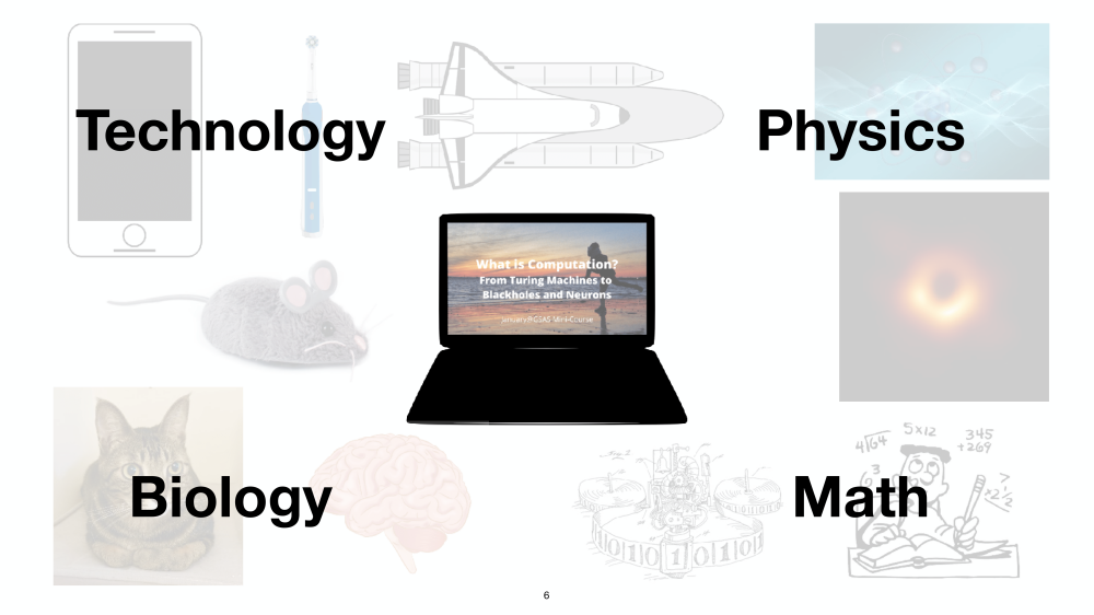
What is Computation?
From Turing Machines to Black Holes and Neurons
Harvard GSAS Mini-Course, January 2022
Update [01/30/2022]: This mini-course had been over but you can access all the recordings here. Comments and suggestions are welcomed!
GSAS Event Page: link.
Meeting Time: January 10-14 & January 17-21 10:00am-11:50am Eastern Time.
Google Calendar: link.
Blog Post: link.
YouTube Playlist: link.
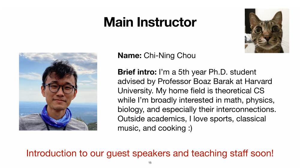
Instructor: Chi-Ning Chou (he/him/his; they/them/theirs)
Guest Speakers:
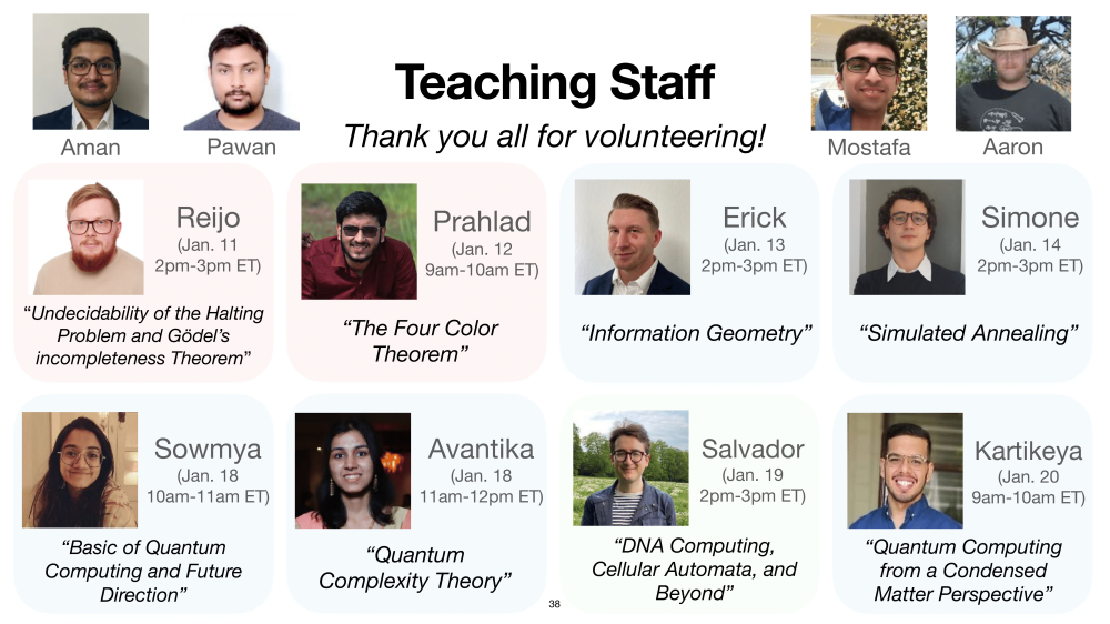
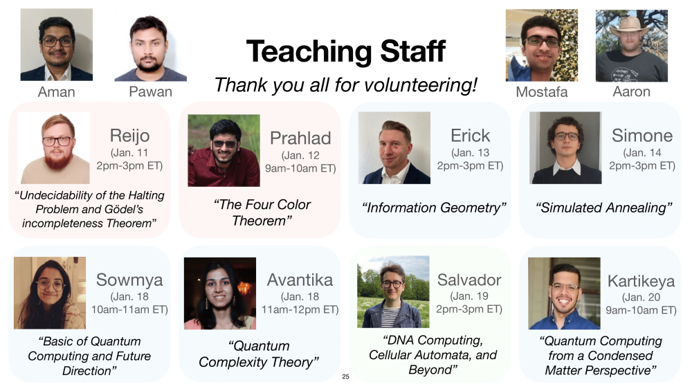
Teaching Staff: Avantika Agarwal, Kartikeya Arora, Salvador Buse, Aaron K. Clark, Erick Galinkin, Simone Maria Giancola, Aman Goel, Reijo Jaakkola, Pawan Mishra, K Prahlad Narasimhan, Tirukkovalluri Sri Sowmya, Mostafa Touny.
Course Description
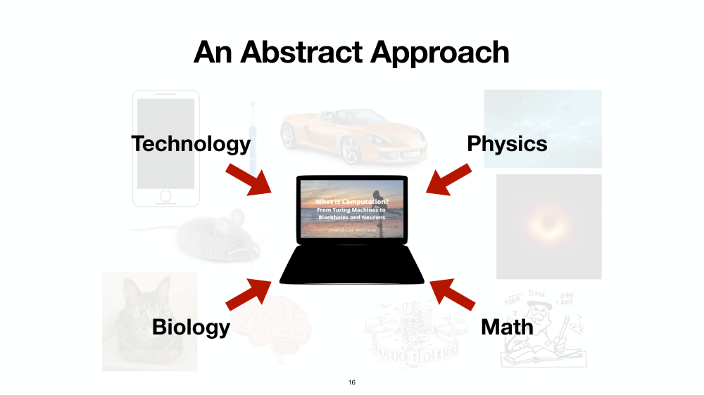
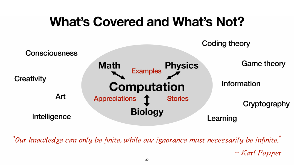
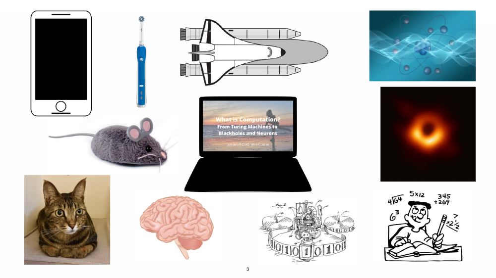
Overview: We are in the era of computation. Everything from a spacecraft to your digital toothbrush has a computer inside it. Meanwhile, physicists told us that physical systems such as black holes are doing some kind of computation and neuroscientists told us our intelligence is built on top of small computations by neurons. What do they really mean by computation therein? Does computation mean the same thing in different fields? Furthermore, do we really understand what computation is?
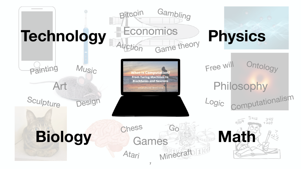
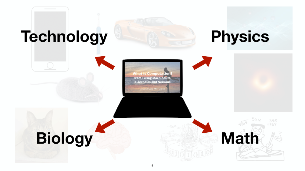
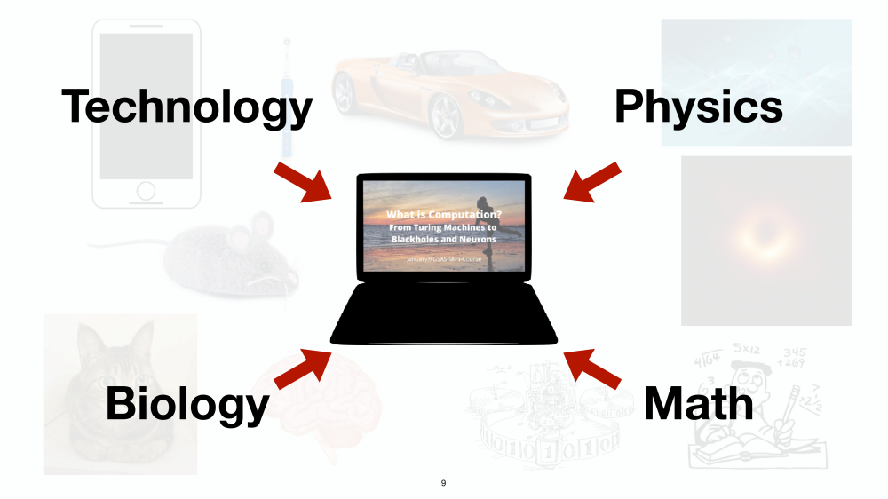
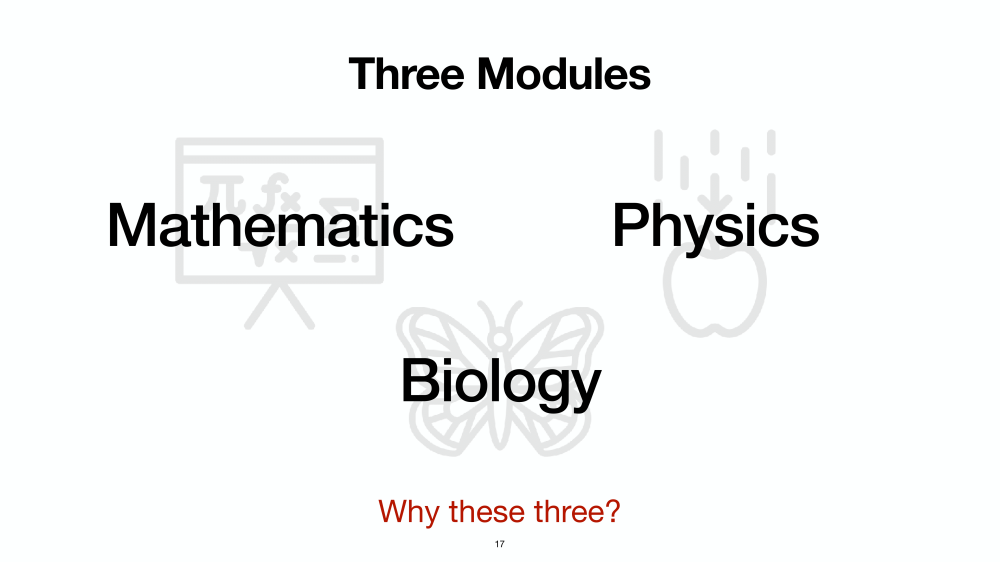
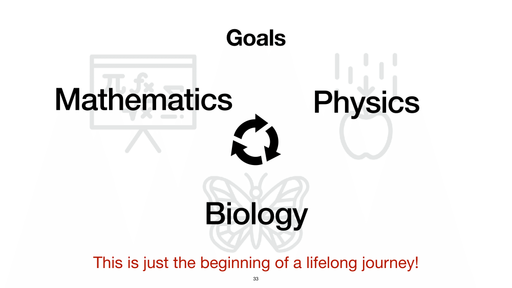
In this mini-course, we are going to revisit the concept of computation through three different perspectives starting from mathematics, to physics and biology. Through theories, examples, and experiments, we are going to see the similarities and differences between these disciplines. The aim of this mini-course is to remind people of the diverse nature of computation and envision the possibilities of future interdisciplinary research.
There will be three modules and each contains three 50-minute interactive lectures and 1-3 guest talk(s). The first module focuses on the mathematical foundation of computations in which the students will learn the concept of Turing machines, computability, reductions, and most importantly, the underlying philosophy. The second module is about the computations in the physical world where we will launch from classical mechanics, to statistical mechanics, quantum mechanics, and gravity. The third module looks into the computations in biology, ranging from genomes, evolution, to neuroscience.
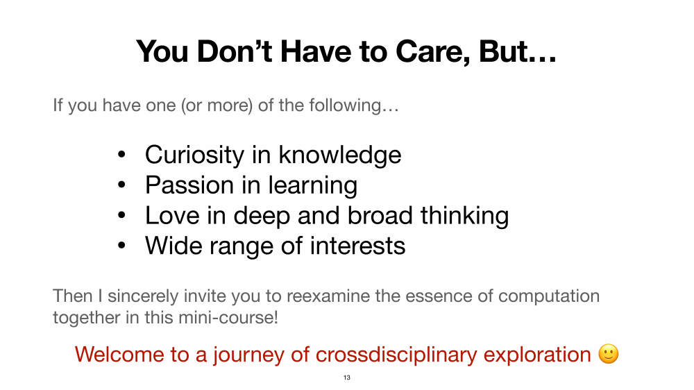
Prerequisites: No math or science prerequisites are required but we expect the students to be comfortable with seeing simple equations. We are particularly welcoming students from any background. The only requirement is having the willingness to communicate with and being respectful to people from different backgrounds.
Policies and expectations: We expect students to attend as many lectures and activities as possible. We will send out a survey one week prior to the mini-course for students’ availability and potentially adjust the times accordingly. Another survey for students to commit on their attendance (don’t need to commit to all the activities!) will be sent out once the lecture & lab times have been finalized.
Learning outcomes: By the end of the course, we hope that the students will all be able to:
- Understand the high-level story of each topic and be able to explain to non-experts.
- Appreciate and respect the different ways of thinking from different fields and perspectives.
- Comfortably communicate with people from different backgrounds.
- Build up interests in some of the topics and perhaps be willing to study further in the future.
The main components of the course are as follows:
- Main class meetings: These will be interactive lectures, with the exposition and discussion guided by student questions and comments.
Labs: These will be simple experiments demonstrating the key concepts learned in the class. We also welcome creative and artistic elements brought by the students! (The in-person labs got cancelled due to the latest COVID regulations)- Guest talks: These will be invited talks given by Ph.D. students or postdocs from relevant fields. The aim is to let the students have exposure to frontier research and thinking in each field.
- Coffee chats: These will be informal casual chatting sessions with free coffee and snacks made by the instructor. Due to the latest COVID regulations, this might not happen.
- The Panel discussion (new): Near the end of the mini-course, we will host a panel discussion for the students to interact with every guest speaker and the lecturer.
- Advanced sections (new): Outside the main lectures, the teaching staff will offer several 1-hour advanced sections covering a wide range of topics related to the course materials.
Topics
The course is composed of one introductory lecture, one concluding lecture, and three modules: (I) The mathematical foundation of computation; (II) Computations in the physical world; (III) Computations in the biological world. Each module will contain three 50-minute lectures where two of them (indexed by a,b) focus on theory and examples while the other (indexed by c) talks about philosophy and methodology. Each module will also have a lab and a guest talk.
- Introductory Lecture: Motivation; Overview; Goal; Logistics. [slides] [video].
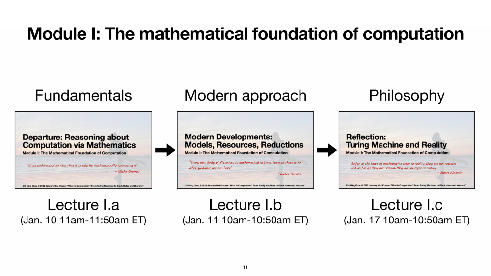
Module I: The mathematical foundation of computation
Is there any problem that a mathematician cannot solve? This is known as Hilbert’s 10th problem and was one of the most important mathematical problems in the beginning of the 20th century. Intriguingly, the answer turned out to be negative. In fact, most of the problems in the mathematical world are unsolvable! To put this into a bigger context, the resolution of Hilbert’s 10th problem was a corollary of Turing’s great achievement of establishing the mathematical foundation of computation.
In this module, students will learn Turing’s mathematical formalization of computation as well as the two other central notions in the modern study of computation: asymptotics and reductions. Other computational notions such as non-determinism, randomness, and communications will also be discussed. The goal is to provide intuitions for students to think about the mathematical formulation of computation and be able to compare with the materials covered in the next two modules.
- Lecture I.a (Departure: Reasoning about Computation via Mathematics): Computational problems; Hilbert’s problems; Turing machines; Uncomputability Theorem. [slides] [video].
- Lecture I.b (Modern Developments: Models, Resources, Reductions): Other computational models; Circuits; Communication; Other computational resources; Nondeterminism; Randomness; Reductions; Cook-Levin Theorem; KW Games. [slides] [video].
- Lecture I.c (Reflection: Turing Machine and Reality): Mathematical Church-Turing Thesis; Philosophy of computation; Philosophy of science. [slides] [video].
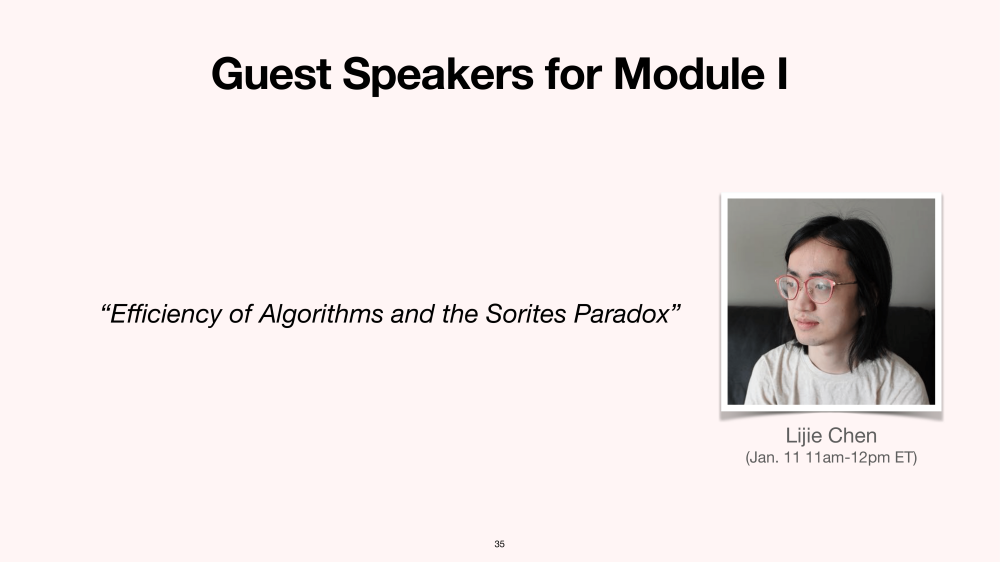
Lab I: Have fun with reductions.- Guest talk I.a: Lijie Chen on “Efficiency of Algorithms and the Sorites Paradox”. [video] [abstract ]
Why do theoretical computer scientists think of an algorithm with running time $100000n$ being efficient while another with running time $2^{n/100000}$ being inefficient? In this talk, I'm going to introduce you to a philosophical foundation of this central formalism in theoretical CS. I will guide you to rethink about the definition of "efficient algorithm" through the lens of Sorites paradox. Furthermore, we will touch on connections to Moore's law, cosmology, and beyond. Hope that after the talk, you won't feel that you are old when you wake up tomorrow! (if you didn't get this joke, you will after attending my talk!)
Gödel’s incompleteness theorems are milestone results in mathematical
logic and they have deep implications to foundations of mathematics.
The first incompleteness theorem essentially states that there does not
exists a Turing machine which can enumerate all the true statements of
number theory, while the second incompleteness theorem demonstrates
that no formal theory which covers all of mathematics (such as ZFC)
can prove its own consistency.
A surprising and not well-known aspect of the first incompleteness
theorem is that it can be derived by simply using the fact that the Halting problem of Turing machines is an undecidable problem. Furthermore, the resulting proof is more transparent (and accessible) than Gödel’s original proof.
In this lecture we will indicate how Gödel’s first incompleteness
theorem can formalized and give an outline for an argument that proves
it. In the course of formalizing it we will also take a closer look at
first-order logic and proof systems. We will also briefly discuss the
background of Gödel’s incompleteness theorems, Gödel’s original proof
for the first incompleteness theorem and the second incompleteness
theorem.
Consider a map of a country. For aesthetic reasons, it makes sense to strive for neighboring states (or provinces) to be colored using different colors. At the same time, using too many colors might be expensive to print and confusing. Therefore, we ask the following question: what is the minimum number of colors that I need to color a certain map? Intuitively, you might expect that the larger the map the more colors you would need. In this talk, we take a look at a remarkable result called the "Four-Color Theorem" which states that any map can be colored with at most four colors. We explore the historical significance of the problem and dip our toes into the key ideas behind the proof that had evaded mathematicians for over a century. Finally, we will look at the ripples that this proof created in the mathematical circles; as the first major result highly reliant on computers, it presented a watershed moment in mathematics: What is a mathematical proof? Can computers prove theorems? Does mathematics lose its credibility if it uses computers?
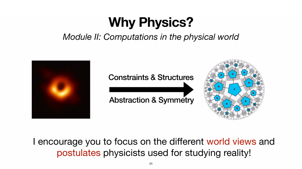
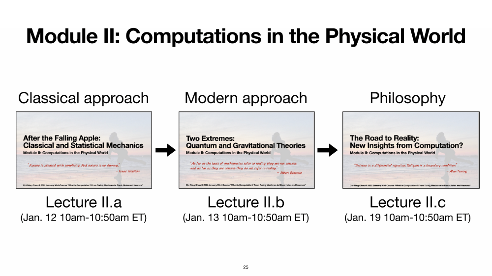
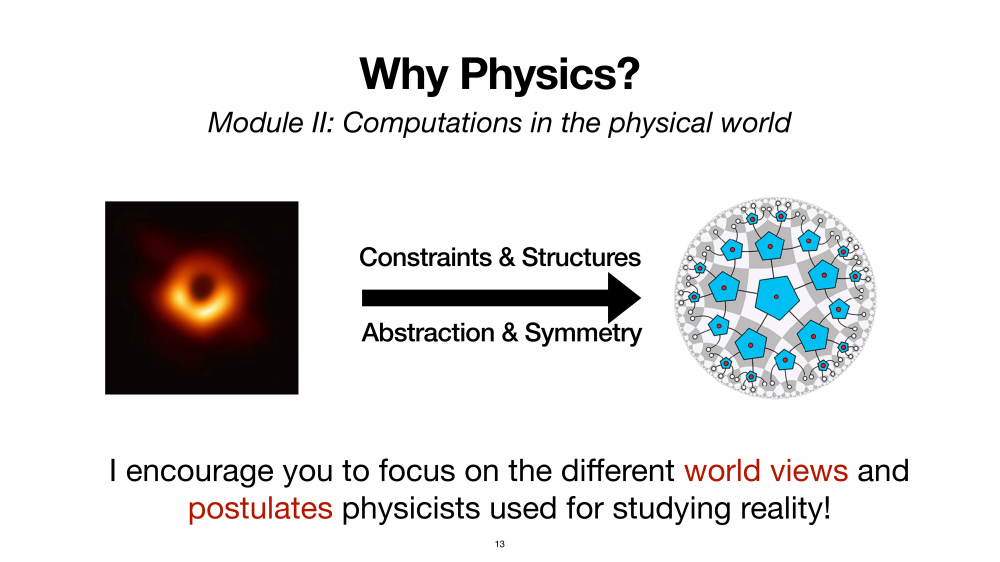
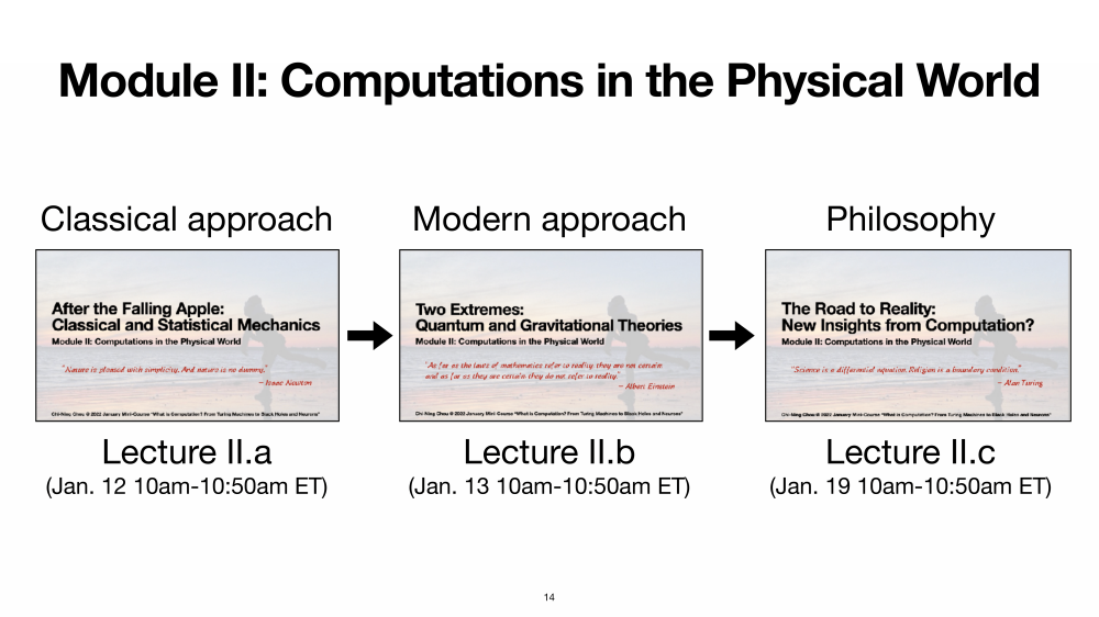
Module II: Computations in the physical world
Well before the apple falling on to Newton’s head, physicists had been searching for the underlying laws that govern reality. These beautiful mathematical descriptions explain how the stars move in a certain pattern, how small particles interact with each other, and so on. But “why” are these physical laws governing the universe rather than others? “What” are these physical laws doing and is there any underlying “problem” they are solving?
In this module, we are going to explore these questions through the lens of computation. Students will learn the basics of classical mechanics, statistical physics, quantum mechanics, and theory of gravity and peek into the connection to computation via “energy minimization” and “entropy maximization”. The goal is to (i) learn how physicists think, (ii) compare the concept of computations in the physical world to the mathematical formulation discussed in module 1, and (iii) build up sufficient language and knowledge for the next module.
- Lecture II.a (After the Falling Apple: Classical and Statistical Mechanics): Lagrangian and Hamiltonian mechanics; Statistical physics [slides] [video].
- Lecture II.b (Two Extremes: Quantum and Gravitational Theories): Quantum mechanics; Gravity and black holes [slides] [video].
- Lecture II.c (The Road to Reality: New Insights from Computation?): Pancomputationalism; Computation in physical systems; Physical Church-Turing Thesis; MIP*=RE [slides] [video].
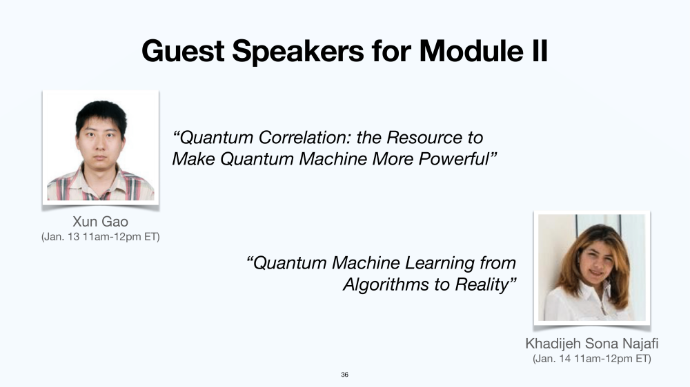
Lab II: Gravity circuits.- Guest talk II.a: Xun Gao on “Quantum Correlations: the Resources Making Quantum Machines More Powerful”. [abstract ]
In this lecture, I will give an overview about the topic of quantum correlations. Quantum correlation is the statistical results produced by measuring quantum system which cannot be produced by classical physics (in general, stochastic process, equivalently hidden variable theory in terms of quantum foundation research or ontological model in terms of philosophy). Concretely, I will discuss very briefly about quantum entanglement, quantum non-locality (the correlation caused by entanglement) and quantum contextuality (a generalization of quantum non-locality). Then I will mention very briefly about a potential application of quantum correlation to machine learning models. Knowledge of quantum mechanics/quantum information is not required.
The computational paradigms of machine learning and quantum computing are different; machine learning tries to find the optimal solution in a heuristic way, while quantum computing harnesses the quantum laws allowing for more efficient and powerful computation as compared to classical computers. With the recent progress both in quantum computing and machine learning, we have entered into a realm that has not been explored before. In particular, while reaching the fault tolerance quantum computing requires another milestone, the question of whether we can gain an advantage by merging these technologies remains crucial. Thus within the realm of current noisy hardware and machine learning which are known to be robust to noise, in this talk, we first discuss three generations of quantum machine learning, each harnessing a particular aspect of quantum computers and targeting particular problems. The first scrutinize the power of quantum computers to work with high dimensional data and speed up algebra. The second generation circumvents the input/output problem by using a hybrid architecture, performing optimization on a classical computer while evaluating parameterized states on a quantum circuit, chosen based on a particular problem. Subsequently, the third generation is inspired by brain-like computation and uses the natural interaction and unitary dynamic of a given quantum system as a source for learning. After introducing each category, we provide examples from those algorithms and show the learning of several cognitive tasks such as multitasking, decision making, and long-term memory by taking advantage of several key features of quantum hardware.
The scientific community has long focused on finding efficient methods for solving problems. However, certain instances present a structure that does not allow finding an exact solution with the present knowledge and technology. Building on this, the attempts moved towards finding a probabilistically acceptable solution, with a change of orientation towards error analysis and reliability. Simulated Annealing is a method that achieves such a philosophy of thought by approximating in a clever way highly complex problems. It is a perfect example of inspiration from nature and thinking out of the box. In the lecture, we will show why such a system might be needed, and then derive directly an instance of the Algorithm step by step.
- Advanced section II.c: Tirukkovalluri Sri Sowmya on “Basic of Quantum Computing & Future Directions”. [video].
- Advanced section II.d: Avantika Agarwal on “Quantum Complexity Theory”. [video]. [abstract ]
Quantum computers are known to provide exponential speedups in solving certain problems, compared to the best known classical algorithms. While we know interesting results in this direction, for example, Simon's algorithm, we have also seen Grover's algorithm, which provides a "much less exciting" polynomial speedup. Is this the best possible improvement?
To address this question, in this talk, we will look at the "limitations" of quantum computers. In particular, we see a technique for proving that indeed some problems are "difficult" to solve on a quantum computer.
I have used many informal terms in this abstract, which will be formalised during the talk. It is recommended to attend the previous talk which introduces quantum computing, before this talk. If you are however unable to attend (or you know the basics of quantum computing already), I will introduce the required basics again at the start of my talk. So as long as you know high school mathematics, you are good to go!
- Advanced section II.e: Kartikeya Arora on “Quantum Computing from a Condensed Matter Perspective”. [video]. [abstract ]
Condensed Matter Physics is ubiquitous in almost all fields of science and technology. From superconductivity to topological phases to actual quantum computers, condensed matter covers it all. In this talk, I'll cover the basics of Quantum Mechanics, Condensed Matter Physics, and Tensor Networks. I'll also try to motivate
the need for quantum computers from a condensed matter physics perspective. As a bonus, I am going to talk about time crystals and give you a recipe to create one for yourself too. Although I'll try to review the basics, it'll be better if you have attended the previous talks on quantum computing (or have some previous experience).
- Advanced section II.f: Chi-Ning Chou on “When Black Holes Meet Computational Complexity”. [video]. [abstract ]
In Lecture II.b, it was hinted that there are several computational aspects of black holes relevant to resolving paradoxes in quantum gravity. In this advanced section, we are going to give a more formal treatment on these connections. I will start with setting up the mathematical language and formally describe the information paradox as well as the firewall paradox. Then, I'll explain a proposal of resolving these paradoxes through the lens of computational complexity and the critics to this approach. Although there will be more math involved in this talk, the high-level story should still be very approachable to the general audience.
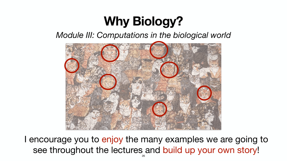
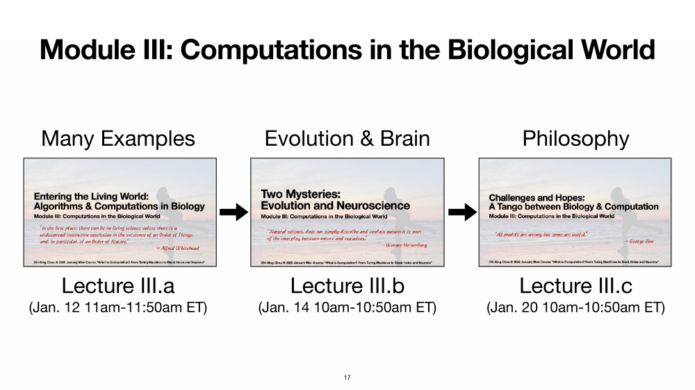
Module III: Computations in the biological world
Biology is the study of life. What is life? How does life form? What is the purpose of life, if there’s any? Unlike physics and mathematics, the challenges of reproducibility in biology, e.g., emergence properties and the precision in experiments, make it an extremely difficult subject to study. Statistical methods have been a prominent approach to establish biological knowledge while in recent years computational methods have arisen as a new angle to understand the biological world. Through the tango between biology and computation, how can the two inspire each other?
In this module, students will see various examples of the computational aspects of biology, including genomes, evolution, neuroscience, etc. The goal is to envision how the computational view can enrich understanding in biology and vice versa. In particular, we will be focusing on the open-ended nature of the living world and compare it with the previous two modules.
- Lecture III.a (Entering the Living World: Algorithms and Computations in Biology): What is Living Science; Computational Biology; Biological Computation [slides] [video].
- Lecture III.b (Two Mysteries: Evolution and Neuroscience): Evolution; Neuroscience [slides] [video].
- Lecture III.c (Challenges and Hopes: A Tango between Biology and Computation): Open-endedness; Emergence; The challenge and difficulty of studying biology; Mathematical ineffectiveness in biology [slides] [video].
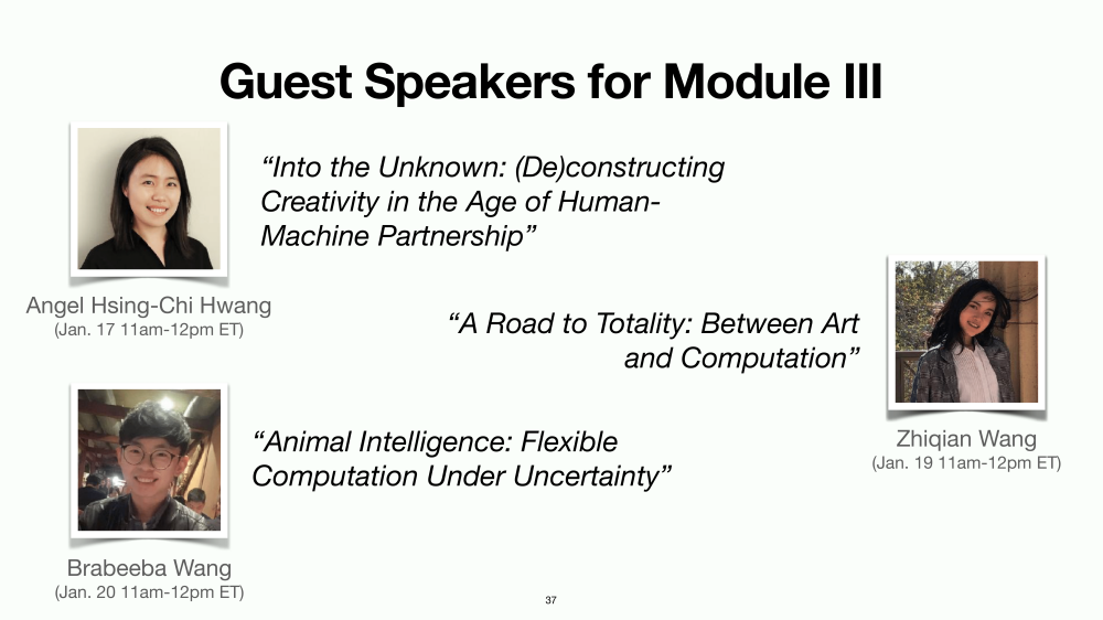
Lab III: Computation and intelligence in slime mold.- Guest talk III.a: Angel Hsing-Chi Hwang on “Into the Unknown: (De)constructing Creativity in the Age of Human-Machine Partnership”. [video]. [abstract ]
It has become clear that machines — and specifically artificial intelligence — will play a critical role in the future of work. When we vision the blueprint of future human-machine collaboration, should our bot partners get involved in innovation or should we guard creativity as “the last territory of humanity”? In this lecture, we introduce the various constructs of human creativity and how they have been studied, measured, quantified, and even sequenced in multiple disciplines. Together, we discuss how, why, and whether machines can learn and practice creativity.
What is art? What is the nature of beauty? Is beauty in the eyes of the beholder or is beauty eternal? If we regard each individual’s experience in viewing or creating art as a computational process, what insights can we bring to this elusive question through a different angle? In this talk, I will give you a tour from caveman’s arts to Duchamp’s urinal and explore the potential connections between art and computation.
What’s intelligence? Is it memory, abstract reasoning or creativity? In this talk, we will dive in on the philosophical aspects of intelligence and attempt to give a working definition of intelligence. We will also give a few examples on different approaches in neuroscience to study intelligence.
- Advanced section III.a: Salvador Buse on “Computing with Chemistry: Turing Machines, Graph Colouring, and DNA”. [video]. [abstract ]
In this talk, I hope to convince you that we can think of chemical reactions as a programming language, which we can use to write any algorithm we choose. I will introduce two different models of chemical reactions — bulk reactions and stochastic reactions — and show how these can execute analog and digital logic, including the emulation of Turing machines. Finally, I will explain how we can compile chemical reactions to DNA, and introduce the field of DNA computing.
- Concluding Lecture: Summary; Students’ Sharings; A Warning and a Wish. [slides] [video].
Materials & Resources
The instructor will provide slides and additional notes available on the course website after each lecture. Optional readings and resources will also be posted on the course website. Before the course begins, we also encourage students to take a look at some of the references listed below.
Module I: The mathematical foundation of computation
Articles:
- Horswill, Ian. “What is computation?”, 2008, link.
- Wigderson, Avi. “The Godel Phenomenon in Mathematics: A Modern View.” Kurt Gödel and the Foundations of Mathematics (2011): 475, link.
- Davis, Philip J. “Toward a Philosophy of Computation.” For the Learning of Mathematics 3.1 (1982): 2-5, link.
- Knuth, Donald E. “Computer science and its relation to mathematics.” The American Mathematical Monthly 81.4 (1974): 323-343, link.
Introductory Books:
- Moore, Cristopher, and Stephan Mertens. The nature of computation. OUP Oxford, 2011, link.
- Barak, Boaz. Introduction to Theoretical Computer Science. Online, link.
- Rautenberg, Wolfgang. A concise introduction to mathematical logic. New York, NY: Springer, 2006, link.
Advanced Books:
- Wigderson, Avi. Mathematics and computation. Princeton University Press, 2019, link.
- Arora, Sanjeev, and Boaz Barak. Computational complexity: a modern approach. Cambridge University Press, 2009, link.
Fun reads:
- Aaronson, Scott. “Why philosophers should care about computational complexity.” Computability: Turing, Gödel, Church, and Beyond 261 (2013): 327, link.
Module II: Computations in the physical world
Articles:
- Preskill, John. “Quantum computing 40 years later.” arXiv preprint arXiv:2106.10522 (2021), link.
- Gualtiero Piccinini and Corey Maley. “Computations in Physical Systems.” Stanford Encyclopedia of Philosophy, 2010, link.
- Yao, Andrew Chi-Chih. “Classical physics and the Church–Turing thesis.” Journal of the ACM (JACM) 50.1 (2003): 100-105, link.
- Piccinini, Gualtiero and Corey Maley, “Computation in Physical Systems”, The Stanford Encyclopedia of Philosophy (Summer 2021 Edition), Edward N. Zalta (ed.), link.
Introductory Books:
- Feynman, Richard P., Tony Hey, and Robin W. Allen. Feynman lectures on computation. CRC Press, 2018, link.
- Penrose, Roger. The road to reality: A complete guide to the laws of the universe. Random house, 2005, link.
- Mezard, Marc, and Andrea Montanari. Information, physics, and computation. Oxford University Press, 2009, link.
Advanced Books:
- Mézard, Marc, Giorgio Parisi, and Miguel Angel Virasoro. Spin glass theory and beyond: An Introduction to the Replica Method and Its Applications. Vol. 9. World Scientific Publishing Company, 1987, link.
- Sakurai, Jun John, and Eugene D. Commins. “Modern quantum mechanics, revised edition.” (1995): 93-95, link.
- Alber, Gernot, et al. Quantum information: An introduction to basic theoretical concepts and experiments. Vol. 173. Springer, 2003, link.
Module III: Computations in the biological world
Articles:
- Schnitzer, M. Biological computation: Amazing algorithms. Nature 416, 683 (2002), link.
- Chelly Dagdia, Z., Avdeyev, P. & Bayzid, M.S. Biological computation and computational biology: survey, challenges, and discussion. Artif Intell Rev 54, 4169–4235 (2021), link.
- Piccinini, Gualtiero. “Computationalism.” The Oxford handbook of philosophy of cognitive science. 2012, link.
Books:
- Nowak, Martin A. Evolutionary dynamics: exploring the equations of life. Harvard university press, 2006, link.
- Jones, Neil C., Pavel A. Pevzner, and Pavel Pevzner. An introduction to bioinformatics algorithms. MIT press, 2004, link.
- Gillespie, John H. Population genetics: a concise guide. JHU Press, 2004, link.
Fun reads:
- Stanley, Kenneth O., and Joel Lehman. Why greatness cannot be planned: The myth of the objective. Springer, 2015, link.
- Schrödinger, Erwin. What is life?: With mind and matter and autobiographical sketches. Cambridge university press, 1992, link.
- Mayr, Ernst. This is biology : the science of the living world. Harvard University Press, 2001, link.
- Banatre, Jean-Pierre, et al., eds. Unconventional Programming Paradigms: International Workshop UPP 2004, Le Mont Saint Michel, France, September 15-17, 2004, Revised Selected and Invited Papers. Vol. 3566. Springer Science & Business Media, 2005, link.
FAQs
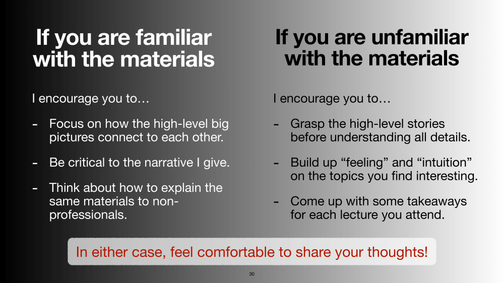
Q: If I don’t have a strong math and science background, what will I learn and will there be any difficulties?
A: Most of the lectures will focus on the high-level stories and the underlying philosophy so will be very accessible to anyone! The instructor will also make sure more knowledgeable students won’t dominate the discussion and create a friendly environment.
Q: What if I already know most of the materials, what will I get from this course?
A: If this is the case, we encourage you to talk to us in advance. In general, the course materials won’t touch the details of each subject and instead focus on high-level stories and comparison with each other. This should provide you with new angles and insights into the subjects you originally were familiar with. Advanced and extra reading/reference materials will be provided on request.
Q: Is there homework for the mini-course?
A: No, but we will provide food-for-thought questions and brainstorming problems at the end of each lecture.
Q: Will all the lectures be recorded?
A: Yes, the recording link will be sent out once available and in long term will be posted somewhere publicly.