Basic Communication Complexity
Basically, the note follows the flow of the classic textbook by Arora and Barak, a fantastic survey by Razborov, and a nice survey on disjointness by Chattopadhyay and Pitassi.
The two-party communication model
In a two-party communication model, the goal is to compute a boolean function $f:\bit^n\times\bit^n\rightarrow\bit$ where one of the input $x\in\bit^n$ is held by Alice and the other input $y\in\bit^n$ is held by Bob. During the communication, Alice and Bob will follow a predetermined protocol and send messages to each other. The communication complexity is defined as the minimum bits required in the protocol that computes $f$.
- For convenience, here we introduce the deterministic protocol first.
- For convenience, here we consider the case where the two inputs have the same length.
- Alice and Bob have unbounded computation power. Thus, undecidable language such as halting problem could be solved under this computation model.
Let $f:\bit^n\times\bit^n\rightarrow\bit$. A deterministic communication protocol $P$ for $f$ is a sequence of functions $(g_1,\dots,g_t)$ such that for any $x,y\in\bit^n$, for any $i=0,1\dots,t$,
- ($i$ is odd) Alice sends Bob $m_i=g_i(x,m_2,m_4,\dots,m_{i-1})$.
- ($i$ is even) Bob sends Alice $m_i=g_i(y,m_1,m_3,\dots,m_{i-1})$.
Furthermore, $m_t=f(x,y)$. Also, define the complexity of $P$ as $CC(P):=\sum_{i\in[t]}\card{m_i}$.
Let $f:\bit^n\times\bit^n\rightarrow\bit$. The deterministic communication complexity of $f$ is defined as \begin{equation} D(f) := \min_{P\text{ computes }f}C(P). \end{equation}
As a result, our goal would be characterizing the communication complexity of arbitrary function. Concretely, to
- upper bound $D(f)$, one need to explicitly find a protocol that computes $f$ and to
- lower bound $D(f)$, one need to somehow argue that for any protocol with less than certain communication complexity will fail on computing certain input.
The history (transcript) of a protocol
A useful concept in communication complexity is the history (or transcript) of a protocol.
Let $P$ be a communication protocol and $x,y\in\bit^n$ be the inputs. Define the history (or transcript) or $P$ on executing $(x,y)$ as $h_{P,x,y}=(m_1,m_2,\dots,m_t)$.
A trivial upper bound
For deterministic two-party communication model, we have $D(f)\leq n+1$ for any $f$ due to the following protocol:
- Alice sends $x$ to Bob.
- Bob computes $f(x,y)$ and sends the outcome to Alice.
Some common functions
- Equality: $\text{EQ}_n$
\begin{equation} \text{EQ}_n(x,y)=\mathbf{1}_{\forall i\in[n],x_i=y_i}. \end{equation}
- Disjointness: $\text{Disj}_n$
\begin{equation} \text{Disj}_n(x,y)=\mathbf{1}_{\forall i\in[n],x_i\cdot y_i\neq1}. \end{equation}
- Inner product: $\text{IP}_n$
\begin{equation} \text{IP}_n(x,y)=\sum_{i\in[n]}x_i\cdot y_i\ (\text{mod }2). \end{equation}
Some lower bound techniques
Let me first give a high-level overview to the lower bound techniques of communication complexity.
All of the known techniques have the following strategy:
- Identify a combinatorics/algebraic property of $f$.
- Show that the number of bits used in a protocol of $f$ can give a upper (or lower) bound for that property.
- Thus, the property of $f$ (or its inverse) can be a lower bound for the number of bits of any protocol for $f$, i.e., the communication complexity of $f$.
When studying the lower bound techniques below, it would be nice to keep in mind the high-level strategy and identify what kind of property being used in the proof.
The rectangle lemma
Before we formally introduce a bunch of lower bound techniques, let’s take a look at a very useful lemma.
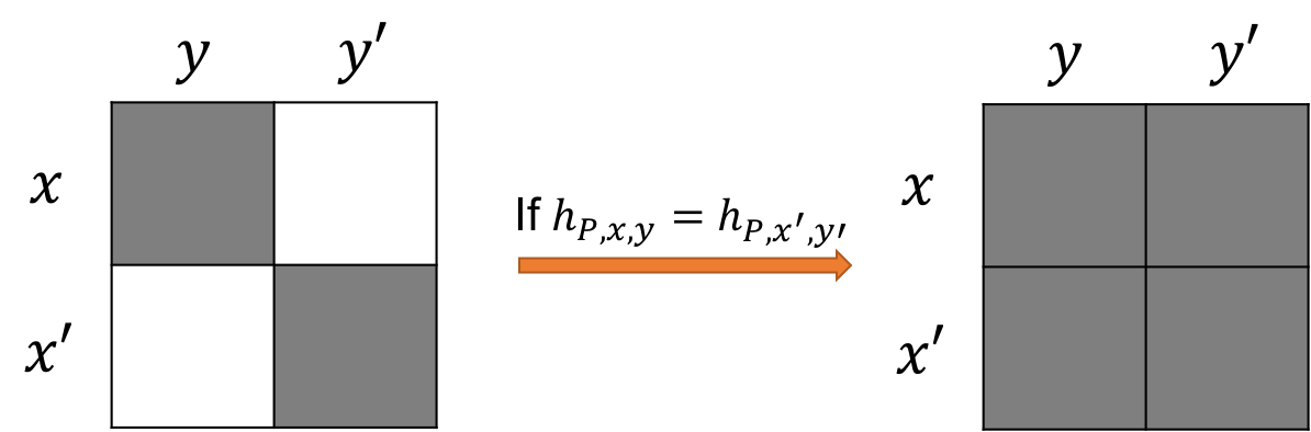
Let $P$ be a deterministic two-party protocol, suppose $h_{P,x,y}=h_{x’,y’}=h$, then $h_{P,x,y’}=h_{x’,y}=h$.
It suffices to prove $h_{P,x’,y}=h$. In the following, we denote the history at the $i$th round on input $(x,y)$ as $(h_{P,x,y})_i$.
In the first round, Alice sends $g_1(x)=g_1(x’)=m_1$ to Bob. That is, $(h_{P,x,y})_1=(h_{P,x’,y’})_1=(h_{P,x’,y})_1$.
In the $i$th round,
- ($i$ is odd) Alice sends Bob
\begin{align}
&g_i(x,(h_{P,x,y})_2,(h_{P,x,y})_4,\dots,(h_{P,x,y})_{i-1})\\
&=g_i(x’,(h_{P,x’,y})_2,(h_{P,x’,y})_4,\dots,(h_{P,x’,y})_{i-1}) \end{align} - ($i$ is even) Bob sends Alice
\begin{align}
&g_i(y,(h_{P,x,y})_1,(h_{P,x,y})_3,\dots,(h_{P,x,y})_{i-1})\\
&=g_i(y,(h_{P,x’,y})_1,(h_{P,x’,y})_3,\dots,(h_{P,x’,y})_{i-1}) \end{align}
Intuitively, the rectangle lemma can be illustrated with the following figure:
Fooling set method
The fooling set method is best illustrated by the equality function $EQ_n$ where $EQ_n(x,y)=\mathbf{1}_{x=y}$ for any $x,y\in\bit^n$. The following lemma says that $(x,x)$ and $(y,y)$ have different communication history.
For any protocol for $EQ_n$ and inputs $x\neq y\in\bit^n$, $h_{P,x,x}\neq h_{P,y,y}$
Suppose $h_{P,x,x}=h_{P,y,y}$, we will show that $h_{P,x,y}=h_{P,y,x}=h_{P,x,x}$ and thus $f(x,y)=f(y,x)=1$, which is a contradiction to the definition of $EQ_n$. The analysis is based on the following rectangle lemma.
By the rectangle lemma, if $h_{P,x,x}=h_{P,y,y}$, then $h_{P,x,y}=h_{P,x,x}$ and thus $f(x,y)=1$, which is a contradiction.
From the above lemma, we have that $S=\{h_{P,x,x}:\forall x\in\bit^n\}$ is of cardinality $2^n$. As a result, $t$ should be at least $n$ otherwise the number of distinct history won’t be enough. We summarize the technique into the following lemma.
We call $S=\subseteq\bit^n\times\bit^n$ a fooling set of boolean function $f$ if the following two conditions hold:
- For any $(x,y)\in S$, $f(x,y)=1$.
- For any $(x,y)\neq(x’,y’)\in S$, it cannot be the case that $f(x,y’)=f(x’,y)=1$.
For any boolean function $f$ with fooling set $S$, we have $D(f)\geq\log\card{S}+1$.
By the rectangle lemma, for any two distinct elements in the fooling set, their history should be different. That is, it requires $\card{S}$ distinct histories for the fooling set. Moreover, as the answer of elements in the fooling set are all the same and the last bit is used to summit the answer, any valid protocol for $f$ requires at least $\log\card{S}+1$ communications.
The number of distinct histories upper bound the size of a fooling set.
Tiling method
To motivate the tiling method, let’s view the deterministic two-party communication protocol in a combinatorics way as follows.
Suppose the protocol $P$ uses at most $k$ bits, then for each $h\in\bit^k$, define $S_{P,h}:=\{(x,y)\in\bit^n\times\bit^n:\ h_{P,x,y}=h\}$ that contains all the input pairs whose communication history is $h$. Let $X_{P,h}:=\{x:\ \exists y\text{ s.t. }(x,y)\in S_{P,h}\}$ and $Y_{P,h}:=\{y:\ \exists x\text{ s.t. }(x,y)\in S_{P,h}\}$. By the rectangle lemma above, we have for any $x\in X_{P,h}$ and $y\in Y_{P,h}$, $(x,y)\in S_{P,h}$. Namely, $S_{P,h}=X_{P,h}\times Y_{P,h}$. Let’s formulate the above idea as follows.
Let $S$ be a set. For any $X,Y\subseteq S$, we say $X\times Y$ is a combinatorics rectangle of $S\times S$.
We can see that the $X_{P,h}\times Y_{P,h}$ defined above is exactly a combinatorics rectangle of $\bit^n\times\bit^n$. Furthermore, the function $f$ has the same value in each rectangle $X_{P,h}\times Y_{P,h}$. We call them monochromatic rectangles.
For any boolean function $f:\bit^n\times\bit^n\rightarrow\bit$ and $X,Y\subseteq\bit^n$, we say $X\times Y$ is a $f$-monochromatic rectangle if for any $x\in X$ and $y\in Y$, $f(x,y)$ has the same value.
Finally, observe that $X_{P,h}\times Y_{P,h}$ is a $f$-monochromatic rectangle for any $h$ and $\{X_{P,h}\times Y_{P,h}:\ \forall h\}$ actually partitions $\bit^n\times\bit^n$. We call such partition a monochromatic tiling.
For any boolean function $f:\bit^n\times\bit^n\rightarrow\bit$. We say $T\subseteq\{X\times Y:\ X,Y\subseteq\bit^n\}$ is a $f$-monochromatic tiling if
- for any $X\times Y\in T$, $X\times Y$ is a $f$-monochromatic rectangle,
- for any $X\times Y\neq X’\times Y’\in T$, $X\times Y$ and $X’\times Y’$ are disjoint, and
- for any $x,y\in\bit^n$, there exists $X\times Y\in T$ such that $(x,y)\in X\times Y$.
Furthermore, define $\chi(f)$ as the least number of rectangles in a $f$-monochromatic tiling.
With the above formal definitions, we can immediately see that a protocol $P$ for $h$ forms a $f$-monochromatic tiling $\{X_{P,h}\times Y_{P,h}:\ \forall h\}$. That is, we have an immediate lower bound for $D(f)$ w.r.t. $\chi(f)$.
For any boolean function $f:\bit^n\times\bit^n\rightarrow\bit$. $D\geq\log\chi(f)$.
However, the other direction, finding a protocol with a $f$-monochromatic tiling,is not so clear. The state-of-the-art upper bound is the following.
For any boolean function $f:\bit^n\times\bit^n\rightarrow\bit$. $D(f)=O(\log^2\chi(f))$.
There exists a function $f$ such that $D(f)\geq\log^{2-o(1)}\chi(f)$.
The number of histories upper bound the number of rectangles in a monochromatic tiling.
Rank method
The main idea of rank method is to view a function $f:\bit^n\times\bit^n\rightarrow\bit$ as a matrix defined as follows.
Let $f:\bit^n\times\bit^n\rightarrow\bit$ and pick an arbitrary ordering over $\bit^n$. Define $M_{f}$ as a $2^n\times 2^n$ matrix where for each $i,j\in[2^n]$, $(M_{f})_{ij}=f(x_i,x_j)$.
- Note that the ordering of $\bit^n$ does not affect the rank of a matrix.
It turns out that $\log\rank(M_f)$ is a lower bound for $D(f)$.
For any $f:\bit^n\times\bit^n\rightarrow\bit$. We have $D(f)\geq\rank(M_f)$. In fact, we have $\chi(f)\geq\rank(M_f)$.
Let $T=\{X_1\times Y_1,\dots,X_k\times Y_k\}$ be the optimal tiling of $f$. Denote the indicator vector of $X\subseteq[n]$ as $\mathbf{1}_{X}$ such that $(\mathbf{1}_X)_i=1$ iff $x_i\in X$. We have
\begin{equation} M_{f} = \sum_{i\in[k]:\ f(x,y)=1,\forall x\in X_i,y\in Y_i}\mathbf{1}_{X_i}\mathbf{1}_{Y_i}^{\intercal}. \end{equation}
As a result, \begin{equation} \rank(M_f)\leq\card{\{i\in[k]:\ f(x,y)=1,\forall x\in X_i,y\in Y_i\}}\leq\chi(f). \end{equation}
Discrepancy method
Comparison of these lower bound techniques
By definition, the tiling method is no weaker than the fooling set method and the rank method. Moreover, there exists gap instance among them(TODO).
Other models
| Functions | Deterministic | Bounded Randomized | Unbounded Randomized | Public Coin | Quantum |
|---|---|---|---|---|---|
| $\text{EQ}_n$ | $\Theta(n)$ | $O(\log n)$ | $\leq2$ | $\leq2$ | |
| $\text{promise-EQ}_n$ | $\Theta(n)$ | $\Theta(n)$ | $\Theta(n)$ | $O(\log n)$ | |
| $\text{Disj}_n$ | $\Theta(n)$ | $\Omega(n)$ | $O(\log n)$ | $O(\sqrt{n}\log n)$ | |
| $\text{IP}_n$ | $\Theta(n)$ | $\Omega(n)$ | $\Omega(n)$ | $\Omega(n)$ |
Nondeterministic
In the nondeterministic communication model, the protocol is given a string $w$ that can be before the execution.
Randomized
In the randomized communication model, both Alice and Bob have unbiased coin that they can use during the computation. For a randomized communication protocol $P$, on input $x$ and $y$, we denote the probability of successfully computing the correct output as $p_{P,x,y}$. We define the randomized communication complexity of $f$ as follows.
- (bounded error randomized communication complexity) $R(f):=\min_{P,p_{P,x,y}>2/3,\forall x,y}CC(P)$.
- (unbounded error randomized communication complexity) $U(f):=\min_{P,p_{P,x,y}>1/2,\forall x,y}CC(P)$.
- (zero error randomized communication complexity) $R_0(f):=\min_{P,p_{P,x,y}=1,\forall x,y}CC(P)$.
Also, we can define the public coin randomized communication complexity in the same way as $R^{pub}(f),U^{pub}(f),R^{pub}_0(f)$ where the protocol is allowed to use public coin. Concretely, we can model the public coin randomized communication model as flipping the coin in advance and put in on a black board that can be accessed by everyone.
Bounded randomized
- $R(\text{EQ})=O(\log n)$
The protocol is based on polynomial identity testing. Think of the bits of Alice and Bob as the coefficients of a degree $n-1$ polynomials. Namely, $A(t)=\sum_{i\in[n]}x_it^{i-1}$ and $B(t)=\sum_{i\in[n]}y_it^{i-1}$.
Distributional
In the distributional communication model, the input pair $(x,y)$ is coming from a distribution $\mu$. We say a deterministic protocol $P$ is valid for $f$ in the distributional communication model w.r.t. $\mu$ if the probability of correctly computing $f$ is at least $2/3$. Furthermore, we denote $D^{\mu}(f)$ as the minimum communication complexity of any valid deterministic protocol for $f$ w.r.t. $\mu$.
For any $f$ and $\epsilon,\delta>0$, $R_{\epsilon+\delta}(f)\leq R^{pub}_{\epsilon}(f)+O(\log\frac{n}{\delta})$.
Distributional v.s. Randomized
The following is a direct relations among randomized communication complexity and distributional communication complexity.
For any $f$, $\mu$, and $\epsilon>0$, \begin{equation} R_{\epsilon}(f)\geq R^{pub}_{\epsilon}(f)\geq D^{\mu}_{\epsilon}(f), \end{equation} That is, to lower bound randomized communication complexity, it suffices to lower bound the distributional complexity for any $\mu$.
The first inequality is trivial. The second inequality follows by designing a deterministic protocol by hard-wiring the good public-coin. By averaging argument, we know that there exists a realization of public-coin that correctly computes the value of $f$ for at least $1-\epsilon$ of input pairs w.r.t. $\mu$. As a result, the success probability of this deterministic protocol w.r.t. $\mu$ is at least $1-\epsilon$.
Concretely, let $P(x,y,r)$ be a public-coin randomized protocol for $f$ with error at most $\epsilon$, we have for any $x,y\in\bit^n$, \begin{equation} \bbP_{R}[P(x,y,R)=f(x,y)]\geq1-\epsilon. \end{equation} Let $X,Y$ be sampled from $\mu$, we have \begin{equation} \bbP_{(X,Y)\leftarrow\mu,R}[P(X,Y,R)=f(x,y)]\geq1-\epsilon. \end{equation} As a result, by averaging argument, there exists $r$ such that \begin{equation} \bbP_{(X,Y)\leftarrow\mu}[P(X,Y,r)=f(x,y)]\geq1-\epsilon. \end{equation} Thus, $P(\cdot,\cdot,r)$ would be a deterministic protocol for $f$ with error at most $\epsilon$ w.r.t. $\mu$.
Furthermore, there’s a even tighter connection among them.
For any $f$ and $\epsilon>0$, $R^{pub}_{\epsilon}(f)=\max_{\mu}D^{\mu}_{\epsilon}(f)$.
The idea is viewing the choice of protocol and the distribution as a two-player zero-sum game. Thus, by applying von Neumann’s min-max theorem, the theorem follows.
Concretely, let player 1 chooses the deterministic protocol $P$ and player 1 chooses the input $(x,y)$. Define the payoff matrix $A$ as $A_{P,(x,y)}=1$ iff $P(x,y)=f(x,y)$. Note that
- A randomized strategy of player 1 is a public-coin protocol.
- A distribution on the choice of $(x,y)$ is a randomized strategy of player 2.
- Given a deterministic protocol $P$ and a distribution $\mu$ on the choice of $(x,y)$, $\mathbf{1}_{P}^{\intercal}A\mu$ is the success probability of $P$ w.r.t. $\mu$. Here $\mathbf{1}_{P}$ is the indicator vector for $P$.
- Given a randomized strategy of player 1 denoted as vector $\sigma$ and an input pair $(x,y)$, $\sigma^{\intercal}A\mathbf{1}_{(x,y)}$ is the success probability of the randomized public-coin protocol on input pair $(x,y)$.
As a result, as we assume $\max_{\mu}D^{\mu}_{\epsilon}(f)\leq c$ for some $c$, we have \begin{equation} \min_{\mu}\max_{\sigma}\sigma^{\intercal}A\mu\geq\min_{\mu}\max_{P}\mathbf{1}_{P}^{\intercal}A\mu\geq1-\epsilon, \end{equation} where $P$ is any valid deterministic protocol for $f$ with $CC(P)\leq c$ and $\sigma$ is any strategy over these $P$. The first inequality is by the fact that $\{\mathbf{1}_{(x,y)}\subseteq\{\mu\}$. By von Neumann’s min-max theorem, we have \begin{equation} \min_{\mu}\max_{\sigma}\sigma^{\intercal}A\mu=\max_{\sigma}\min_{\mu}\sigma^{\intercal}A\mu\leq\max_{\sigma}\min_{(x,y)}\sigma^{\intercal}A\mathbf{1}_{(x,y)}, \end{equation} where the first inequality is by the fact that $\{\mathbf{1}_P\}\subseteq\{\sigma\}$. Combine the above two we have $\max_{\sigma}\min_{(x,y)}\sigma^{\intercal}A\mathbf{1}_{(x,y)}\geq1-\epsilon$ and thus the maximizaer $\sigma^{*}$ is a public-coin randomized protocol for $f$ that has communication complexity at most $c$ with error at most $\epsilon$. Namely, $R^{pub}_{\epsilon}(f)\leq c$.
Although we have the above tight connection between distributional and public-coin randomized communication model, usually it’s not easy to compute $D^{\mu}(f)$ for arbitrary $\mu$. As a result, basically we will only work on uniform distribution.
Lower bound for distributional communication complexity: The discrepancy method
Recall that a deterministic communication protocol is equivalent to a rectangle-partition on $M(f)$. For a deterministic protocol that is always correct, those rectangles in the partition are monochromatic. What if we allow the rectangle to be non-monochromatic and require the protocol works well with high probability on input sampled from a distribution $\mu$?
The discrepancy of a rectangle captured the probability that the deterministic protocol works well w.r.t. uniform distribution.
Let $R=X\times Y$ where $X,Y\subseteq\bit^n$, the discrepancy of $R$ is defined as \begin{equation} \text{Disc}(R) := \bbP[x\in X,y\in Y]\cdot\card{\bbP[f(x,y)=1|x\in X,y\in Y]-\bbP[f(x,y)=0|x\in X,y\in Y]}. \end{equation}
Multi-party
In a $k$-party communication model, the goal is to commute $f(x_1,\dots,f_k)$ where $f:(\bit^n)^k\rightarrow\bit$ and the $i$th player is given input $x_i$. There are two types of multi-party communication models.
- The Number on Forehead (NOF) model
In the NOF model, each party will put his/her input on the forehead. Namely, they can see the inputs of every party except their own input.
See the following section for an approach to use NOF lower bound to prove $\ACC{0}$ lower bound.
- The Number in Hand (NIH) model
In the NIH model, each player will hide his input. Namely, they can only see their own input.
Quantum
In the quantum communication model, the only difference is that the message between Alice and Bob are qubits instead of classical bits. Similarly, for a quantum communication protocol $P$, we denote the number of qubits in the communication as $CC^Q(P)$. We define the quantum communication complexity of $f$ as follows.
- (bounded error quantum communication complexity) $Q(f):=\min_{P,p_{P,x,y}>2/3,\forall x,y}CC^Q(P)$
- (zero error quantum communication complexity) $Q_0(f):=\min_{P,p_{P,x,y}=1,\forall x,y}CC^Q(P)$.
One can immediately see that $R(f)\geq Q(f)$ and $R_0(f)\geq Q_0(f)$ since one can use quantum to simulate randomized computation.
- For partial functions:
- $R(\text{EQ}’)=\Omega(n)$ and $Q(\text{EQ}’)=O(\log n)$.
- For total functions:
- $R(\text{Disj})=\Omega(n)$ and $Q(\text{Disj})=O(\sqrt{n}\cdot\log n)$.
- There exists a total function $F$ such that $R(F)=\Omega(Q(F)^{2.5})$
See the following section for details.
Applications
It turns out that the lower bound in communication complexity can be used to provide unconditional lower bound in other areas such as space bound of streaming algorithm and depth bound of circuit complexity. In this section, we are going to introduce several classic results.
Space bound of streaming algorithms
Streaming algorithms consider the scenario where the algorithms can only sequentially access the input data once. Concretely, the input would a string over a finite alphabet set $S$ and the goal is to compute certain statistics of that string. The complexity issue is to minimize the space used in the algorithms.
Normally, people are interested in the moments of the input string $x\in S^n$. For instance,
- (the first moment) $m_1:=\sum_{s\in S}\mathbf{1}_{\exists i\in[n],x_i=s}$,
- (the first moment) $m_1:=\sum_{s\in S}\card{\{i\in[n]:x_i=s\}}=n$,
- (the second moment) $m_2:=\sum_{s\in S}\card{\{i\in[n]:x_i=s\}}^2$, and
- (the infinite moment) $m_{\infty}:=\max_{s\in S}\card{\{i\in[n]:x_i=s\}}$.
The following theorem shows that any streaming algorithms for computing the infinite moment requires $\Omega(\card{S})$ space.
Any streaming algorithms for computing the infinite moment over alphabet set of cardinality $n$ requires at least $n$ space.
The high-level idea is to use a streaming algorithm for infinite moment as a black-box in a communication protocol for disjointness.
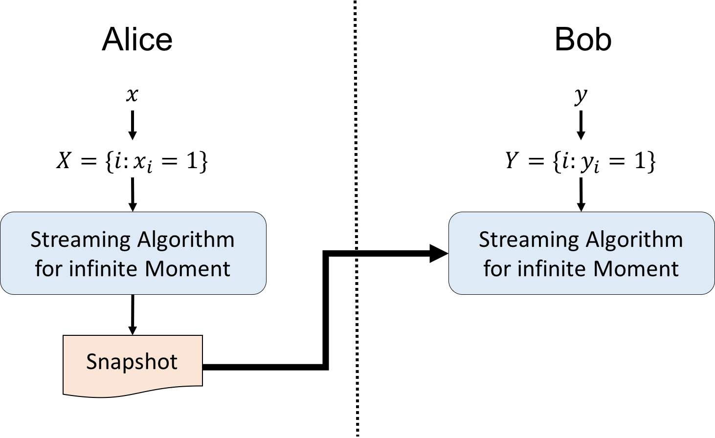
Concretely, each party transform its input $x$ (resp. $y$) to $X=\{i:x_i=1\}$ (resp. $Y=\{i:y_i=1\}$). Alice first feed $X$ as an input to the streaming algorithm over alphabet set $[n]$ and then send the snapshot of the streaming algorithm after the execution to Bob. Bob then execute the streaming algorithm on input $Y$ starting from the snapshot he received from Alice. Finally, if the output is 1, then Bob sends 1 to Alice. Otherwise, Bob sends 0 to Alice.
Note that the output of the streaming algorithm of Bob is equal to the output of the streaming algorithm on input $X\circ Y$. As a result, if $x$ and $y$ are not disjoint, the infinite moment of $X\circ Y$ would be 2. That is, the above protocol can correctly compute the disjointness problem.
Also, by the communication lower bound of disjointness, we know that the bits communicate between Alice and Bob should be at least $n+1$ (including the last bit). That is, the number of bits of the snapshot from Alice should be at least $n$. As a result, we conclude that the streaming algorithm for infinite moment require at least $n$ bits.
Circuit lower bounds
If you are not familiar with circuit complexity, please see this note.
Karchmer-Wigderson game: An exact characterization of circuit depth
The Karchmer-Wigderson game is a communication game that gives an exact characterization of the circuit depth of a function.
The Karchmer-Wigderson game is defined on a function $f:\bit^n\rightarrow\bit$ as follows. There are two players $\ONE$ and $\ZERO$ such that $\ONE$ holds $x\in f^{-1}(1)$ and $\ZERO$ holds $y\in f^{-1}(1)$. The goal of the game is to find some $i\in[n]$ such that $x_i\neq y_i$. Note that as long as $f^{-1}(1)$ and $f^{-1}(0)$ are not empty, there always exists such $i$.
We define $CC_{KW}(f)$ to be the least number of bits required in a communication protocol that solves the Karchmer-Wigderson game for any $x,y$.
The following theorem tells us that $CC_{KW}(f)$ is actually equal to the minimum depth of the circuit that computes $f$!
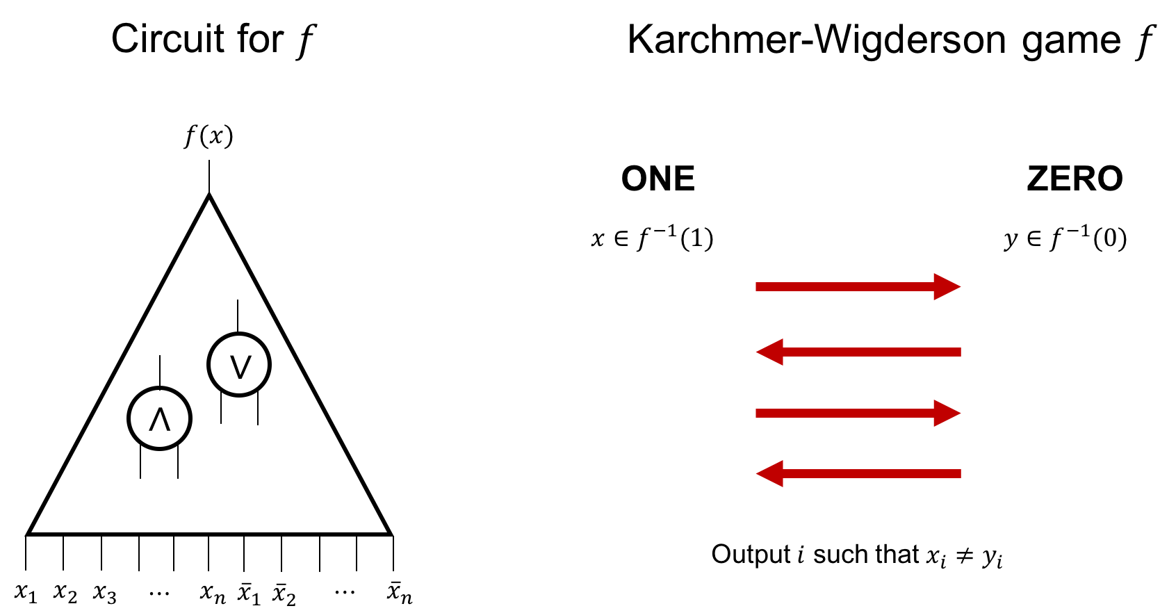
For any $f:\bit^n\rightarrow\bit$, $CC_{KW}(f)$ is exactly the minimum depth of the circuit that computes $f$.
Denote the minimum depth of the circuit that computes $f$ as $d(f)$. Here, we consider the circuit that has no NOT gate and the input gates are $x$ and its negation $\bar{x}$.
- ($CC_{KW}(f)\geq d(f)$): Any depth $K$ circuit computes $f$ can be turned into a $K$ bits communication protocol that solved the Karchmer-Wigderson game.
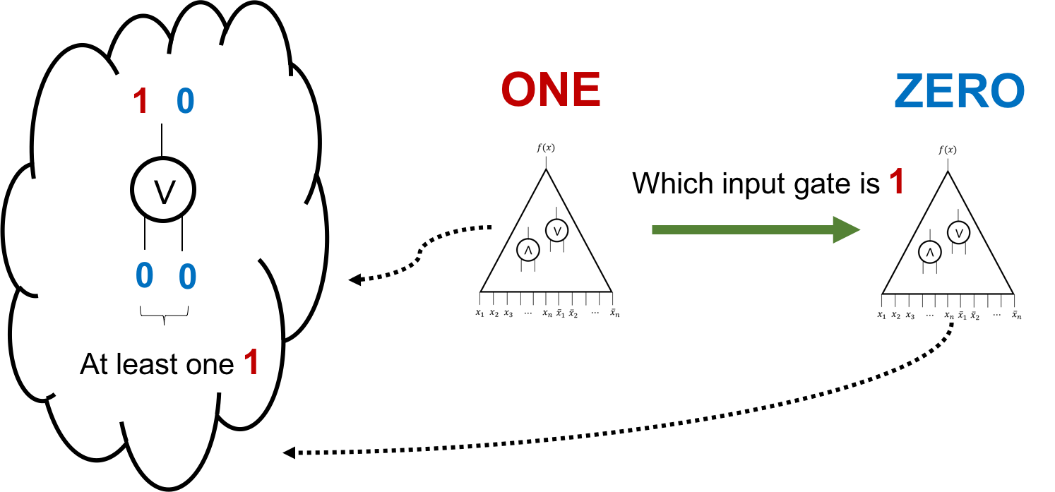
Let $C$ denote the circuit that computes $f$ and has depth $K$. Let’s start from the output gate of $C$. Observe that $\ZERO$ and $\ONE$ have different value on the output gate. The idea is to identify the input gate of this gate (i.e., the output gate) where $\ZERO$ and $\ONE$ still have different value.
- Suppose the gate is an OR gate.
 Observe that
- For $\ZERO$, both the input gates have value 0.
- For $\ONE$, at least one of the input gates has value 1.
Thus, $\ONE$ will send a bit to $\ZERO$ to tell him which input gate has value 1.
- Suppose the gate is an AND gate.
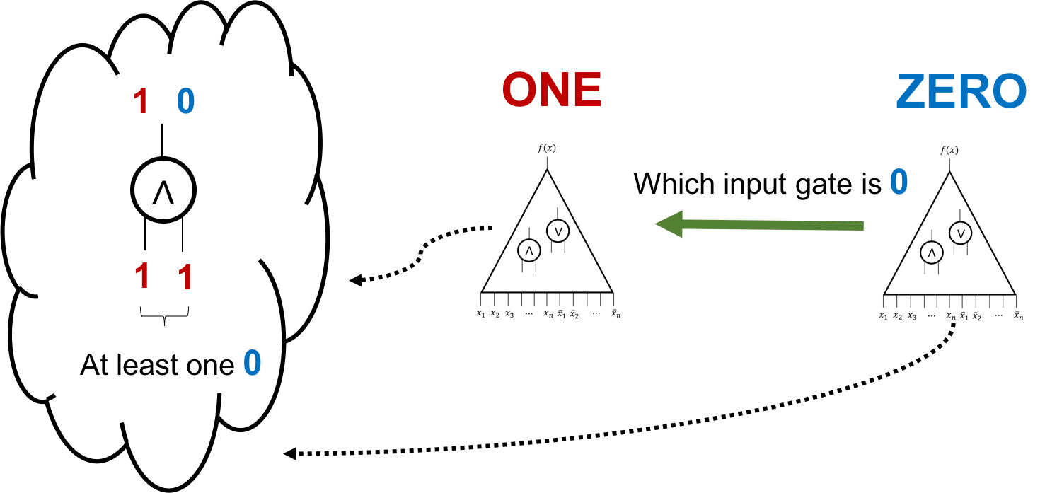
- For $\ONE$, both the input gates have value 1.
- For $\ZERO$, at least one of the input gates has value 0.
Thus, $\ZERO$ will send a bit to $\ONE$ to tell him which input gate has value 0.
Keep repeating the above communication protocol until they reach the bottom layer of $C$. As $\ZERO$ and $\ONE$ always have different value on the gate they agree on. * If they reach the $i$th input bit, then we have $x_i=1$ and $y_i=0$. * If they reach the negation of the $i$th input bit, then we have $x_i=0$ and $y_i=1$.
That is, $x_i\neq y_i$. We have a $K$-bit communication protocol for the Karchmer-Wigderson game of $f$.
- ($d(f)\geq CC_{KW}(f)$): Any $K$ bits communication protocol that solved the Karchmer-Wigderson game can be turned into a depth $K$ circuit that computes $f$.
First, let’s view the Karchmer-Wigderson game as distinguishing two disjoint sets $A,B\subseteq\bit^n$. Denote such game as $KW(A,B)$ and the communication complexity of such game as $CC_{KW}(A,B)$. Namely, $CC_{KW}(f)=CC_{KW}(f^{-1}(1),f^{-1}(0))$.
Let’s prove by induction on the number of bits used in the communication protocol for Karchmer-Wigderson game of $f$.
For the base case, suppose there’s a 0-bit protocol for $KW(A,B)$. Then there must be the case that there exists $i\in[n]$, for any $x\in f^{-1}(1)$, $x_i=1$ (or $x_i=0$) and for any $y\in f^{-1}(0)$, $y_i=0$ (or $y_i=1$). Thus, the circuit for $f$ is simply the $i$th gate or its negation.
Now, suppose there’s a $K$-bit protocol for $KW(A,B)$ where $K>0$. WLOG, suppose $\ONE$ sends $\ZERO$ one bit in the first round of the protocol. Let $A_1\subseteq A$ contains the inputs that $\ONE$ will send 1 to $\ZERO$ and $A_0=A\backslash A_1$. Observe that the rest of the protocol is a $(K-1)$-bit protocol for the $KW(A_1,B)$ or $KW(A_0,B)$ depends on the first bit of $KW(A,B)$.
By induction hypothesis, there exists circuits $C_0,C_1$ of depth at most $K-1$ such that $C_0$ distinguishes $(A_0,B)$ and $C_1$ distinguishes $(A_1,B)$ in the sense that
- If $x\in A_0$, then $C_0(x)=1$.
- If $x\in A_1$, then $C_1(x)=1$.
- If $x\in B$, then $C_0(x)=C_1(x)=0$.
Thus, take $C=C_0\vee C_1$, we have
- If $x\in A$, then $C(x)=1$.
- If $x\in B$, then $C(x)=0$.
That is, $C$ computes distinguishes $(A,B)$. When we take $A=f^{-1}(1)$ and $B=f^{-1}(0)$, $C$ computes $f$.
Thus, we conclude that $CC_{KW}(f)=d(f)$.
Simultaneous NOF model: An approach to find $f\notin\ACC{0}$
In the following, we are going to see how to transform a lower bound for a specific multi-party communication problem to a lower bound for a certain circuit family.
Simultaneous NOF
Let’s first recall the simultaneous NOF communication model. Let $f:(\bit^n)^k\rightarrow\bit$, there are $k$ parties in a simultaneous NOF model for $f$ where on input $x_1,\dots,x_k$, the $i$th player can only see all the inputs except $x_i$. The protocol only has one round where each player simultaneously writes some bits onto a shared blackboard. They then run a deterministic algorithm on the bits written on the blackboard and decide the output. The goal is to correctly compute $f$ while minimizing the number of bits written on the blackboard. Denote the minimum number of bits used in a simultaneous NOF that computes $f$ as $CC_{SNOF}(f)$.
Symmetric 2-layer circuit family
Next, we consider a special circuit family where the circuit only has 2 layers. The first layer consists a symmetric gate that has $s$ fan-in. The second layer consists functions from function family $\mathcal{F}\subseteq\mathcal{F}_t=\{f:\bit^t\rightarrow\bit\}$. We call this family a $(s,\mathcal{F})$-symmetric 2-later circuit family.
Though it looks weird at first glance, the symmetric 2-layer circuit family actually captures some very interesting circuit complexity classes as shown below.
For any function in $\ACC{0}$, there exists a $(n^{\log^{O(1)}n},\mathcal{P}_{n,\poly\log n})$-symmetric 2-layer circuit that computes $f$. $\mathcal{P}_{n,\poly\log n}$ is the family of polynomials over $\bit^n$ of degree at most polylogarithmic in $n$.
Allender shows the first symmetric 2-layer characterization for $\AC{0}$. Yao then shows a probabilistic characterization for $\ACC{0}$. The above result is proved by Beigel and Tarui. We omit the proof here.
The following theorem by Håstad and Goldmann shows an approach to prove $(s,\mathcal{F})$-symmetric 2-layer circuit lower bound via simultaneous NOF communication lower bound.
Let $f:(\bit^n)^k\rightarrow\bit$. Suppose there’s a $(s,\mathcal{F}_{k-1})$-symmetric 2-layer circuit computes $f$, then there exists a simultaneous NOF protocol that computes $f$ with at most $O(k\log s)$ bits. Namely, $CC_{SNOF}(f)=O(k\log s)$.
The goal is to design a simultaneous NOF protocol for $f$ given a $(s,\mathcal{F}_{k-1})$-symmetric 2-layer circuit that computes $f$.
The idea is actually quite simple. First, arbitrarily divide the input $\bit^{n\times k}$ into $k$ parts of equal size and distribute to each party. For each second layer gate, since it depends on at most $k-1$ input bits, there must be some party that knows all the value of the input bits of that gate. Now, each party computes the second-layer gates whose input bits are all available to him and writes the result onto the blackboard. Observe that
- each second-layer gate must be written at least once and
- each party writes at most $\log s$ bits.
As a result, the number of bits used in this protocol is at most $k\cdot\log s$ and thus $CC_{SNOF}(f)=O(k\log s)$.
If $CC_{SNOF}(f)=\omega(k\log s)$, then there’s no size $s$ symmetric 2-layer circuit computes $f$.
Quantum communication complexity
We are going to introduce two classic results:
- For partial functions, there exists an exponential separation between classical and quantum communication complexity.
- For total functions, there exists a quadratic separation between classical and quantum communication complexity.
To complete the proof, we need to establish the following concepts.
View a string as a function
In the following, we will view an input string $x\in\bit^N$ as the truth table of a function $f:\bit^n\rightarrow\bit$ where $N=2^n$.
Black-box quantum computations
In the black-box quantum computation model, there’s a quantum circuit that has oracle access to an input function $f:\bit^n\rightarrow\bit$. The goal is to decide if the function is the yes instance of a language $L$ or not. Denote the minimum number of queries needed for language $L$ as $T_0(L)$ if there’s no error and $T(L)$ if we allow bounded error say $1/3$.
Here we list two languages that are going to be useful in the future.
- (Half or None) Let $\text{BALANCE}$ be the promise problem where $\text{BALANCE}_Y=\{f:f\text{ is balance}\}$ and $\text{BALANCE}_N:\{f:f\text{ is constant}\}$.
$T_0(\text{BALANCE})=1$.
- (Database search) Let $\text{SEARCH}$ be the problem defined as $\text{SEARCH}=\{f:\exists x,\ f(x)=1\}$. Note that we can modify the definition to searching for a 0.
$T_0(\text{SEARCH})=O(\sqrt{N})$.
From computation to communication
In previous work, Buhrman, Cleve, and Wigderson designed a general quantum communication protocol which is embedded with a black-box quantum computation subroutine. As a result, one can translate the results in black-box quantum computation to quantum communication.
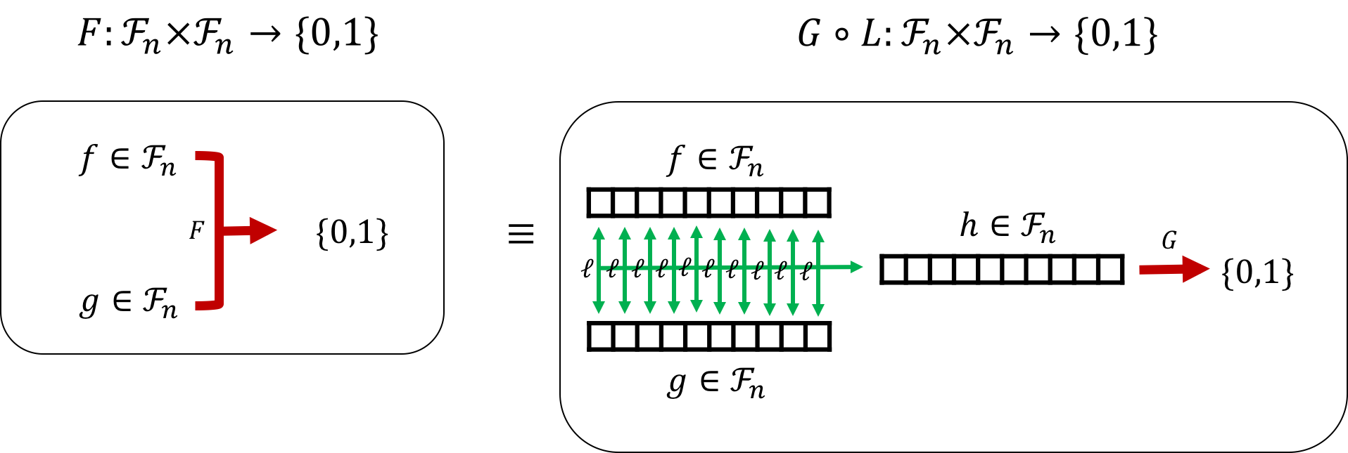
The idea is to rewrite a two-party function $F:\mathcal{F}_n\times\mathcal{F}_n\rightarrow\bit$ into a composition form as $F=G\circ L$ where $G\in\mathcal{F}_n\rightarrow\bit$ and $L:\mathcal{F}_n\times\mathcal{F}_n\rightarrow\mathcal{F}_n$ such that $L(f,g)(x)=\ell(f(x),g(x))$ with $\ell:\bit\times\bit\rightarrow\bit$ for any $f,g\in\mathcal{F}_n$ and $x\in\bit^n$. For instance, let $f=L(f,g)$ for any $f,g\in\mathcal{F}_n$,
- (\text{EQ}) $F(f,g)=G(h)=1$ iff $f$ is a all one function and $\ell$ is the AND gate.
- (\text{Disj}) $F(f,g)=G(h)=0$ iff there exists $x\in\bit^n$ such that $f(x)=1$ and $\ell$ is the NXOR gate.
The following theorem reduce the computing $F$ in the two-party communication model to computing $G$ in black-box model.
Let $F=G\circ L$ defined as above. Suppose $G$ has a black-box algorithm with at most $t$ oracle queries to its input function, then there exists a two-party communication protocol for $F$ that uses at most $t\cdot(2n+4)$ qubits.
Suppose Alice holds function $f\in\mathcal{F}_n$ and Bob holds $g\in\mathcal{F}_n$. The two-party communication protocol for $F$ is designed as follows. Alice runs the black-box algorithm for $G$. Each time the algorithm queries $h=L(f,g)$, say on $x\in\bit^n$, Alice does the following:
- Prepare state $\lvert x\rangle\lvert 0\rangle\lvert 0\rangle$.
- Apply the mapping $\lvert x\rangle\lvert 0\rangle\lvert 0\rangle\rightarrow \lvert x\rangle\lvert 0\rangle\lvert f(x)\rangle$ and send it to Bob.
Bob then applies $\lvert x\rangle\lvert 0\rangle\lvert f(x)\rangle\rightarrow \lvert x\rangle\lvert \ell(f(x),g(x))\rangle\lvert f(x)\rangle$ and sends it back to Alice. Thus, Alice has $h(x)=L(f,g)(x)=\ell(f(x),g(x))$ and is able to proceed the algorithm for $G$.
To sum up, the total communication between Alice and Bob is at most the number of rounds times $(2n+4)$. That is, $t\cdot(2n+4)$.
- $Q_0(\text{EQ}’)=O(\log N)$.
- $Q(\text{Disj})=O(\sqrt{N}\log N)$.
Finally, we end this section with the following two separation theorems.
$Q_0(\text{EQ}’)=O(\log n)$ and $R_0(\text{EQ}’)=\Omega(n)$.
As we have proved quantum upper bound, it suffices to prove classical lower bound.
$Q(\text{Disj})=O(\sqrt{n})$ and $Q_0 (\text{Disj})=\Omega(n)$.
As we have proved quantum upper bound, it suffices to prove classical lower bound.