Basic Counting Complexity
Introduction
Motivation
Maximum likelihood Bayes net
$\ShP$ and $\FP$
Now, let’s formally define the complexity classes for counting problems.
Let $f:\bit^{*}\rightarrow\N$, we say $f\in\FP$ if there exists a Turing machine $M:\bit^{*}\rightarrow\N$ such that for any $x\in\bit^{*}$, $M(x)=f(x)$ and $M(x)$ terminates in $p(\card{x})$ time where $p(\cdot)$ is some polynomial.
Let $f:\bit^{*}\rightarrow\N$, we say $f\in\ShP$ if there exists a Turing machine $M\bit^{*}\times\bit^{*}\rightarrow\N$ such that for any $x\in\bit^{*}$, $f(x) = \card{{y\in\bit^{m(\card{x})}:\ M(x,y)=1 }}$ where $m(\cdot)$ is some polynomial and $M(x,y)$ terminates in $p(\card{x})$ time for some polynomial $p(\cdot)$.
Note that $\FP$ and $\ShP$ are counting analog of the decision complexity classes $\P$ and $\NP$. That is, $\FP$ contains the counting problems that are easily computed while $\ShP$ contains the counting problems that count the number of witnesses.
Is $\ShP$ harder than $\NP$?
If $\CountCycles\in\FP$, then $\P=\NP$.
We prove the theorem by reducing $\HamCycle$ to $\CountCycles$. Namely, we are going to construct a polynomial mapping $f:\mathcal{G}\rightarrow\mathcal{G}$ where $\mathcal{G}$ is the set of graphs. For any graph $G=(V,E)$ where $\card{V}=n$, we have
- If $G\in\HamCycle$, then the number of cycles in $f(G)\geq2^{n^2}$.
- If $G\notin\HamCycle$, then the number of cycles in $f(G)<2^{n^2}$.
One can easily see that if $\CountCycles$ is in $\FP$, then we can compute the number of cycles in $f(G)$ in $\poly(n)$ time, \ie deciding if $G$ has a Hamiltonian cycle in $\poly(n)$ time.
Now, let’s construct $f$ as follows: for any edge $e\in E$, we replace $e$ with the below gadget.

Observe that there are $2^m$ distinct paths from $u$ to $v$ in $f(G)$. That is, when there’s a cycle in $G$ that passes $e$, then the cycle can be duplicated into $2^m$ distinct cycles in $f(G)$. As we replace every edges in $G$ with the gadget above, a cycle $C$ in $G$ can be uniquely mapped to $2^{\card{C}\cdot m}$ cycles in $f(G)$.
Now, we can estimate the number of cycles in $f(G)$.
- If $G\in\HamCycle$, then there’s a cycle of length $n$ in $G$ thus there are at least $2^{n\cdot m}$ cycles in $f(G)$.
- If $G\notin\HamCycle$, the there are at most $n!$ distinct length $n-1$ cycles in $G$. That is, there are at most $n!2^{(n-1)\cdot m}$ cycles in $f(G)$.
As a result, once $2^m>n!$, we can distinguish the two cases. By choosing $m=n^2$, we have $2^{m}>n!$ and thus
- If $G\in\HamCycle$, then the number of cycles in $f(G)\geq2^{n^2}$.
- If $G\notin\HamCycle$, then the number of cycles in $f(G)<2^{n^2}$.
#$\P$-completeness
Let $f:\bit^{*}\rightarrow\N$. We say $f$ is $\ShP$-hard if for any $g\in\ShP$, $g\in\FP^{f}$.
Furthermore, if $f\in\ShP$, then we say $f$ is $\ShP$-complete.
$\ShSAT$ is $\ShP$-complete
Recall that the first complete problem in $\NP$ is the satisfiability problem. So it’s natural to consider $\ShSAT$ as a candidate for $\ShP$-complete problem and it turns out it is.
$\ShSAT$ is $\ShP$-complete.
The idea is based on an observation in the Cook-Levin theorem. Concretely, one can see that the reduction in the Cook-Levin theorem is parsimonious, i.e., the mapping of witnesses is also 1-1 onto.
In Cook-Levin theorem, we consider an arbitrary $\NP$ problem $L$. As $L\in\NP$, it means that there exists a deterministic Turing machine $M$ such that on input $x\in\bit^{*}$ and witness $w\in\bit^{p(\card{x})}$ for some polynomial $p$, $M(x,w)=1$ iff $w$ is a valid witness for $x$.
Next, turn the tableau of $M$ on input $x,w$ into the assignment and turn the local verification of the rules of $M$ into logical gates. We then have a circuit $C_x$ such that an assignment $A$ is a satisfying assignment iff the first $p(\card{x})$ bits encode the witness $w$ of $x$. That is, the number of satisfying assignment of $C_x$ is exactly the same as the number of witnesses of $x$.
Finally, turn $C_x$ into a boolean formula $\phi_x$ such that $A$ is a satisfying assignment for $C_x$ iff $A$ is a satisfying assignment for $\phi_x$. As a result, we conclude that the number of witnesses of $x$ is the same as the number of satisfying assignment of $\phi_x$. In other words, by solving $\ShSAT$, one can solve any problems in $\ShP$.
Valiant’s theorem
$\Permanent$ is $\ShP$-complete.
At first glance, it seems that $\Permanent$ is not a counting problem. However, as we treat the input matrix $A$ as the adjacency matrix of a graph $G_A$, the permanent of $A$ is actually related to the number of weighted cycle covers of $G_A$.
Thus, by constructing special gadget to reduce from $\#\TSAT$ to counting the number of cycle covers, we can prove that $\Permanent$ is $\ShP$-complete.
First, let’s recall the definition of permanent and see its relation to cycle cover.
Let $A\in\bbR^{n\times n}$, define the permanent of $A$ as \begin{equation} \perm(A) := \sum_{\sigma\in S_n}\prod_{i\in[n]}A_{i,\sigma(i)}, \end{equation} where $S_n$ is the group contains all the permutation on $n$ symbols and $\sign(\sigma)$ is the number of switches used in $\sigma$.
Let $G=(V,E)$ be a graph. We say $C=\{C_1,\dots,C_k\}$ is a cycle cover for $C$ if
- $C_i$ is a cycle in $G$ for any $i\in[k]$.
- For any $v\in V$ there exists $C_i$ such that $v\in C_i$.
- $C_1,\dots C_k$ are disjoint to each other.
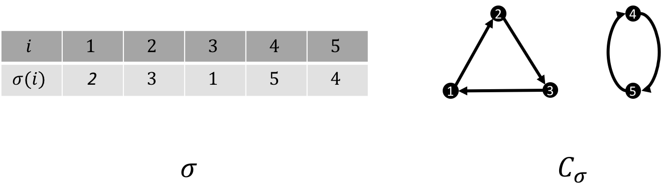
Observe that for each $\sigma\in S_n$, $\sigma$ corresponds to a potential cycle cover for a graph of $n$ vertices and vice versa. Concretely, define $C_{\sigma}$ as follows.
\begin{align}
C_{\sigma} := \{&(i,\sigma(i),\sigma(\sigma(i)),\dots,\sigma^{k-1}(i)) |\ \forall i\in[n],\ k=\min_{t>1}\sigma^t(i)\nonumber\\
&,\ \not\exists 1\leq j<i\text{ such that }\sigma^t(j)=i\text{ for some }t \}.
\end{align}
See the following figure as an example.
From the above observation, we have the following connection between cycle covers and permanent.
Let $A\in\R^{n\times n}$ and $G$ be the weighted graph with adjacency matrix $A$. Then, \begin{equation} \perm(A) = \sum_{C=(C_1,\dots,C_k):\ C\text{ is a cycle cover of }G}\prod_{i\in[k]}\prod_{e=(j_1,j_2)\in C_i}A_{j_1,j_2}. \end{equation}
\begin{align}
\perm(A) &= \sum_{\sigma\in S_n}\prod_{i\in[n]}A_{i,\sigma(i)}\\
&=\sum_{\sigma\in S_n,\ C_{\sigma}=(C_1,\dots,C_k)}\prod_{i\in[k]}\prod_{e=(j_1,j_2)\in C_i}A_{j_1,j_2}\\
&= \sum_{C=(C_1,\dots,C_k):\ C\text{ is a cycle cover of }G}\prod_{i\in[k]}\prod_{e=(j_1,j_2)\in C_i}A_{j_1,j_2}.
\end{align}
Define the problem of summing the weighted cycle covers of a graph as $\CycleCovers$.
By Lemma (connection between permanent and cycle covers), we have the following corollary.
$\CycleCovers\in\FP^{\Permanent}$.
Now, we are going to show that $\ShSAT\in\FP^{\CycleCovers}$ and thus combine with Corollary (Permanent is not easier than Cycle Covers), we have $\Permanent$ is $\ShP$-hard.
$\ShTSAT\in\FP^{\CycleCovers}$.
Let $\phi$ be a $\TSAT$ instance with $n$ variables $x_1,\dots,x_n$ and $m$ clauses $C_1,\dots,C_m$. We are going to define a reduction $f$ from 3CNF to a graph such that \begin{equation} \text{number of cycle covers in }f(\phi) = 9^{\text{number of satisfying assignment of }\phi}. \end{equation}
There are four gadget in the reduction:

Note that there are only two possible cycle covers in the above gadget:
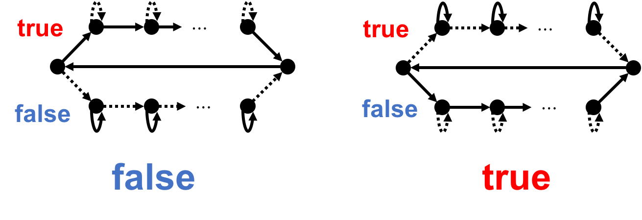 We use real arrow to indicate that the edge was chosen and use dotted arrow to indicate that the edge was not chosen. The above figure illustrates that all the self-loop on the same side must be simultaneously chosen and exactly one side will be chosen.
We call the number of vertices on each side the width of the gadget.

First, note that to have a cycle cover, the three outer edges in an edge gadget cannot be chosen simultaneously. Otherwise, there’s no cycle covers the node in the center. Thus, there are three cases:
- No outer edge
 There are nine possible cycle covers and each of them contributes weight 1.
 - One outer edge
 There are three possible cycle covers each of then contributes weight 3.
 - Two outer edges
 There is one possible cycle cover which contributes weight 9.
Finally, to replace edges of weight 3 with edges of edge 1, we use the following gadget.

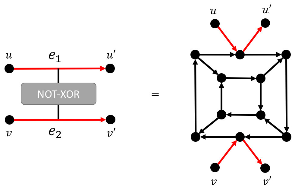
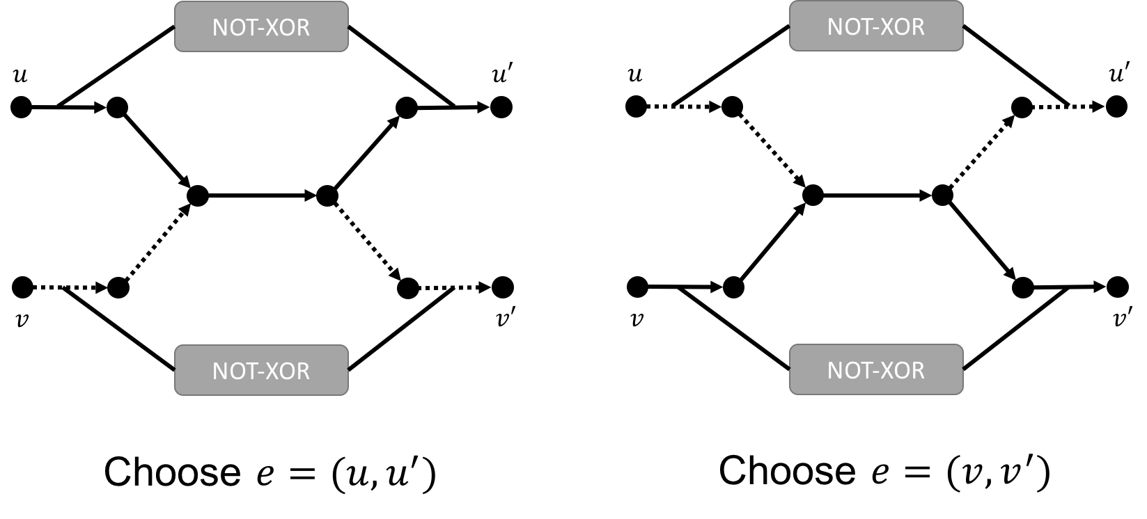
One can see that the two red paths (correspond to the $e_1$ and $e_2$) are either both being chosen or not.
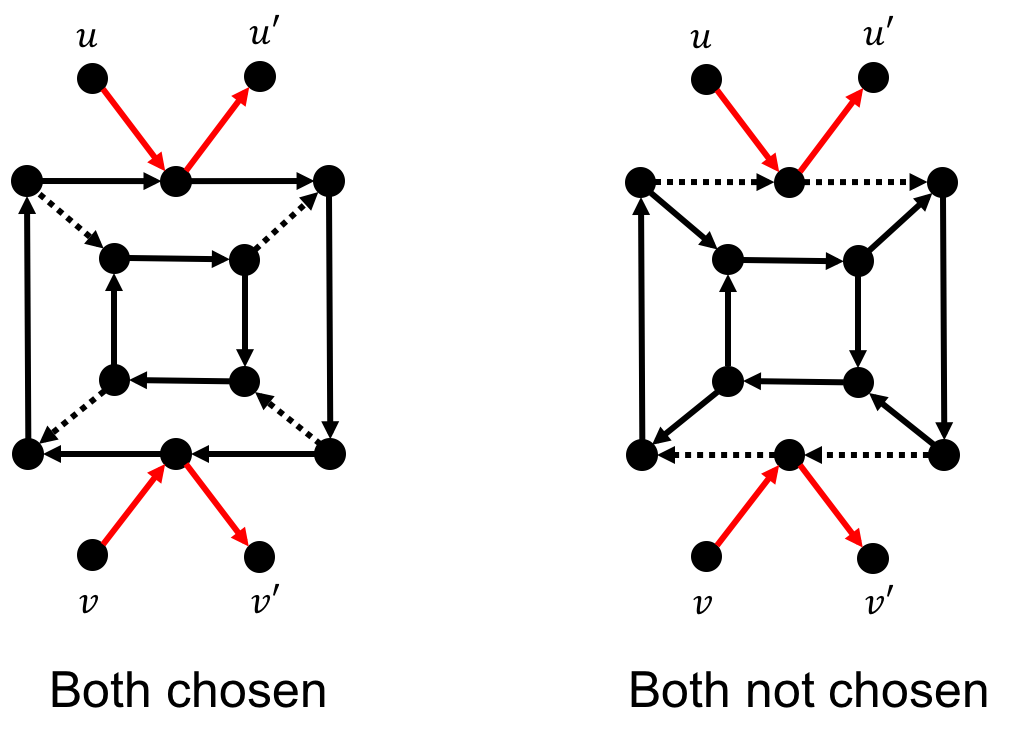
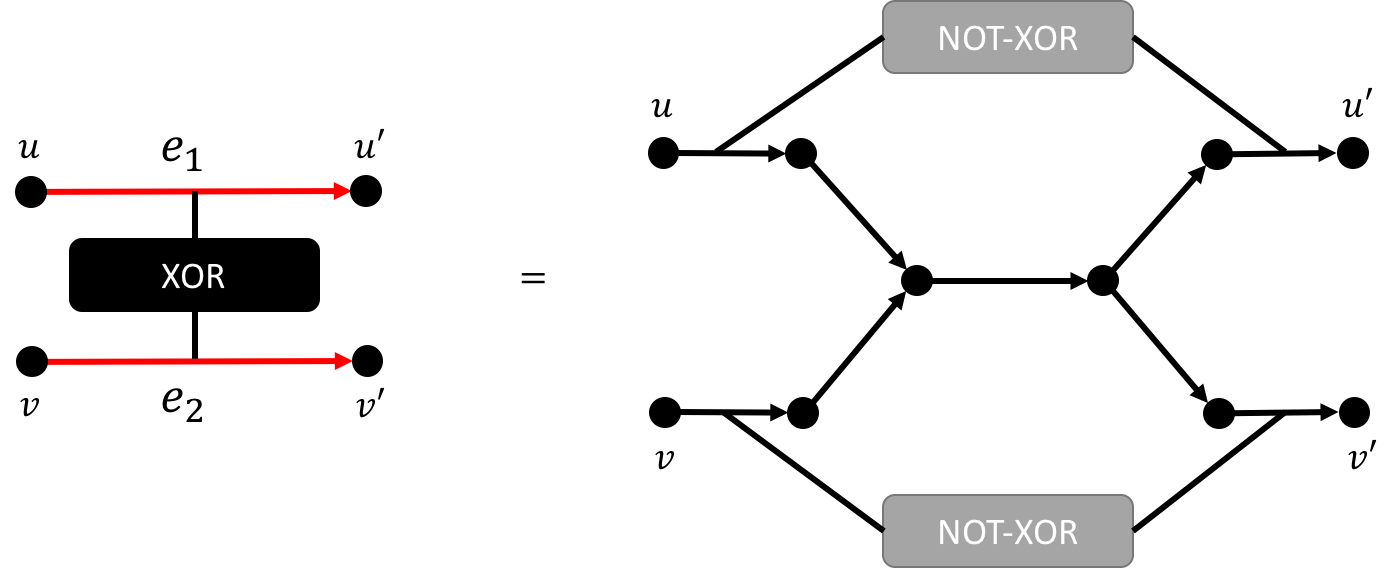
One can see that exactly one of $(u,u’)$ and $(v,v’)$ will be chosen in a valid cycle cover.
Finally, given $\phi(x_1,\dots,x_n)=C_1\wedge\cdots\wedge C_m$ where $C_j=(L_{j,1}\vee L_{j,2}\vee L_{j,3})$ for any $j\in[m]$ and $L_{j,k}=x_i$ or $\neg x_i$ for any $j\in[m],k\in[3]$ for some $i\in[n]$. We reduce $\phi$ to a graph $G_{\phi}$ as follows.
- For each variable $x_i$, $i\in[n]$, associate $x_i$ with a variable gadget of width $m$.
- For each clause $C_j$, $j\in[m]$, associate $C_j$ with an edge gadget.
- Suppose for $j\in[m],k\in[3]$, $L_{j,k}=x_i$, then use the XOR gadget to connect one of the edges in the true side of the $x_i$’s gadget with one of the outer edges of $C_j$’s gadget.
The following is an example of $\phi(x_1,x_2,x_3,x_4)=(x_1\vee\neg x_3\vee x_4)\wedge(\neg x_1\vee\neg x_2\vee x_4)$.
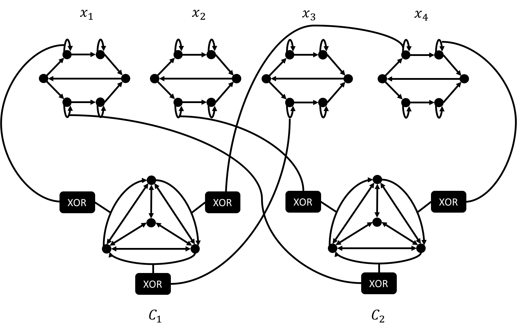
Observe that
- The number of vertices in the $G_{\phi}$ is $n\cdot(2m+2)+m\cdot(4+3\cdot3)+m\cdot3\cdot(6+2\cdot10)=2mn+2n+61m=\poly(n)$.
- A valid cycle cover in $G_{\phi}$ must correspond to a satisfying assignment of $\phi$.
- A satisfying assignment of $\phi$ contributes to exactly $9^m$ distinct cycle covers in $G_{\phi}$.
To sum up, we have \begin{equation} \text{number of cycle covers in }f(\phi) = 9^{\text{number of satisfying assignment of }\phi}. \end{equation}
As a result, we conclude that $\ShTSAT\in\FP^{\CycleCovers}$.
Combine Corollary (Permanent is not easier than Cycle Covers) with Lemma (Cycle Covers is #P-hard), we conclude that $\Permanent$ is $\ShP$-hard. Moreover, as the edges of the graph in the reduction from $\ShTSAT$ to $\FP^{\CycleCovers}$ have 0/1 weight, it also follows that computing permanent of 0/1 matrix is $\ShP$-hard.
Toda’s theorem
It’s natural to compare $\ShP$ with decisional complexity classes. However, as the output formats are different, we need to come up with a way to compare them. A natural candidate is using $P^{\ShP}$. Surprisingly, it turns out that $P^{\ShP}$ contains the whole polynomial hierarchy!
$\PH\in\P^{\#\P}$.
Roadmap
The proof of Toda’s theorem is inspired by a seemingly irrelevant theorem: the Valiant-Vazirani theorem.
- $\SAT\leq_r^{1/8n}USAT$
- $\SAT\leq_r^{1-2^{-O(n)}}\oplus\SAT$
- $\Sigma_k\SAT\leq_r^{1-2^{-O(n)}}\oplus\SAT$
- $\PH\subseteq\P^{\ShP}$
$\SAT\leq_r^{1/8n}USAT$: Valiant-Vazirani theorem
There exists a PPT reduction $A$ such that for any unquantified boolean formula $\phi$ with $n$ variables $\bx$, $A(\phi)$ is an unquantified boolean formula with variables $\bx$ and $\by$ where $\by$ is of $\poly(n)$ length. We have
- If $\phi\in\SAT$, then $\mathbb{P}[A(\phi)\in\USAT]\geq\frac{1}{8n}$.
- If $\phi\notin\SAT$, then $\mathbb{P}[A(\phi)\in\SAT]=0$. Moreover, we can write $A(\phi) = \tau(\bx,\by)\wedge\phi(\bx)$ where the size of $\tau$ is polynomial in $n$.
Given boolean formula $\phi$, let $S:=\{x:\ \phi(x)=1\}$ be the set of satisfying assignments. The idea of Valiant-Vazirani theorem is to probabilistically construct a predicate $B(x)$ such that with non-negligible probability, exactly one element in $S$ satisfies that predicate. As a result, $\phi(x)\wedge B(x)$ will only has exactly one satisfying assignment.
To construct such $B$, let’s start with a simple trial.
- Randomly pick $y\in\bit^n$.
- Let $B_{\text{simple}}=(x=y)$ and output $A_{\text{simple}}(\phi)=\phi\wedge B_{\text{simple}}$.
One can see that
- If $\phi\in\SAT$, then $\mathbb{P}[A_{\text{simple}}(\phi)\in\USAT]\geq\frac{\card{S}}{2^n}$.
- If $\phi\notin\SAT$, then $\mathbb{P}[A_{\text{simple}}(\phi)\in\SAT]=0$.
Note that the completeness here could be exponentially small and is impossible to be amplified.
As a result, hash family turns out to be a natural tool since it can uniformly map the elements from the domain $\bit^n$ to the range $\bit^m$ where $1\leq m\leq n$.
Now, we can construct the predicate as follows.
- Randomly pick $h\in\mathcal{H}_{n,m}$.
- Let $B_{\text{hash}}=(h(x)=0^m)$ and $A_{\text{hash}}=\phi\wedge B_{\text{hash}}$.
One can see that
- If $\phi\in\SAT$, then $\mathbb{E}[\card{\{x:\ A_{\text{hash}}(x)=1\}}]=\frac{\card{S}}{2^{n-m}}$.
- If $\phi\notin\SAT$, then $\mathbb{P}[A_{\text{hash}}\in\SAT]=0$.
Note that the here we only compute the expectation of the size of the intersection of $S$ and the pre-image of the predicate in the completeness part. To compute the probability, we need to specify which hash family we are using. To theoretical computer scientist, the pairwise independent hash family is a randomness-efficient and good enough hash family.
Recall the definition of pairwise independent hash family as follows.
Let $n,m\in\bbN$, $\mathcal{H}_{n,m}\subseteq\{f:\bit^n\rightarrow\bit^m \}$ is a pairwise independent hash family from $\bit^n$ to $\bit^m$ if for any $x\neq x’\in\bit^n$ and $y,y’\in\bit^m$, \begin{equation} \mathbb{P}_{h\leftarrow\mathcal{H}_{n,m}}[h(x)=y\text{ and }h(x’)=y’]=\frac{1}{2^{2m}}. \end{equation}
As we fix the hash family we are using, we can compute the completeness as follows.
Take $m\in[n]$ such that $2^{m-2}\leq\card{S}\leq 2^{m-1}$. If $\phi\in\SAT$, then $\mathbb{P}[A_{\text{hash}}\in\USAT]\geq\frac{1}{8}$.
First, let $S_{A_{\text{hash}}}:= \{x:A_{\text{hash}}(x)=1\}$, by inclusion-exclusion principle, we have
\begin{align}
\mathbb{P}[A_{\text{hash}}\in\USAT] &= \sum_{x\in S_{A_{\text{hash}}}}\mathbb{P}[A_{\text{hash}}(x)=1]\\
&- \sum_{x\neq x’ \in S_{A_{\text{hash}}}}\mathbb{P}[A_{\text{hash}}(x)=1\text{ and }A_{\text{hash}}(x’)=1].
\end{align}
For any $x\in S_{A_{\text{hash}}}$,
\begin{align}
\mathbb{P}[A_{\text{hash}}(x)=1]=\frac{1}{2^m}.
\end{align}
For any $x\neq x’\in S_{A_{\text{hash}}}$,
\begin{align}
\mathbb{P}[A_{\text{hash}}(x)=1\text{ and }A_{\text{hash}}(x’)=1]=\frac{1}{2^{2m}}.
\end{align}
Thus,
\begin{align}
\mathbb{P}[A_{\text{hash}}\in\USAT] &= \card{S_{A_{\text{hash}}}}\cdot\frac{1}{2^m}-\binom{\card{S_{A_{\text{hash}}}}}{2}\cdot\frac{1}{2^{2m}}\\
&\geq\frac{1}{4} - \frac{1}{2}\cdot(\frac{1}{2})^2=\frac{1}{8}.
\end{align}
Finally, uniformly picking $m\in[n]$, we have probability at least $\frac{1}{n}$ such that $2^{m-2}\leq\card{S}\leq2^{m-1}$ and thus the theorem holds.
$\SAT\leq_r^{1-2^{-O(n)}}\oplus\SAT$
Though we got a randomized reduction from $\SAT$ to $\USAT$, however, we cannot amplify the completeness because of the following observation.
- The NO case of $\USAT$ is either unsatisfiable or having more than one satisfying assignment.
- If $\phi\in\SAT$ and $A_{\text{hash}}(\phi)\notin\USAT$, we don’t know whether $A_{\text{hash}}(\phi)$ has zero or more than one satisfying assignments.
But this is not the end of the world, one can see that if we consider the parity of the number of satisfying assignments, then the above obstacles are no longer an issue to worry!
Let $f:\bit^{*}\rightarrow\bit$, we say $f\in\oplus\P$ if there exists a Turing machine $M\bit^{*}\times\bit^{*}\rightarrow\N$ such that for any $x\in\bit^{*}$, $f(x) = \card{{y\in\bit^{m(\card{x})}:\ M(x,y)=1 }}$ mod 2 where $m(\cdot)$ is some polynomial and $M(x,y)$ terminates in $p(\card{x})$ time for some polynomial $p(\cdot)$.
The goal of this step is to show a randomized reduction from $\SAT$ to $\oplus\SAT$.
There exists a PPT $A$ such that for any boolean formula $\phi$,
- If $\phi\in\SAT$, then $\mathbb{P}[A(\phi)\in\oplus\SAT]\geq1-2^{-O(n)}$.
- If $\phi\notin\SAT$, then $\mathbb{P}[A(\phi)\in\oplus\SAT]\leq2^{-O(n)}$.
That is, $\SAT\leq_r^{1-2^{-O(n)}}\oplus\SAT$.
First, given two boolean formulas $\phi(x),\phi’(y)$ that share no common variables, i.e. $x\neq y$, we have
| $\phi$ | $\phi’$ | $\phi\vee\phi’$ |
|---|---|---|
| $\in\oplus\SAT$ | $\in\oplus\SAT$ | $\in\oplus\SAT$ |
| $\in\oplus\SAT$ | $\notin\oplus\SAT$ | $\notin\oplus\SAT$ |
| $\notin\oplus\SAT$ | $\in\oplus\SAT$ | $\notin\oplus\SAT$ |
| $\notin\oplus\SAT$ | $\notin\oplus\SAT$ | $\notin\oplus\SAT$ |
Note that the OR operation on $\phi$ and $\phi’$ does not preserve in the result of parity. As a result, we would like to construct certain operation such that the result of parity can be preserved.
Define the following operations.
- (negation) $\neg^{\oplus}\phi(x):=\phi(x)\vee(z=1\wedge_{i}(x_i=1))$
- (OR) $\phi(x)\vee^{\oplus}\phi’(y):=\neg_{\oplus}(\neg_{(\oplus}\phi(x))\vee\neg_{\oplus}(\phi’(y)))$
- (AND) $\phi(x)\wedge^{\oplus}\phi’(y):=\phi(x)\wedge \phi’(y)$
We have
| $\phi$ | $\phi’$ | $\neg^{\oplus}\phi$ | $\phi\vee^{\oplus}\phi’$ | $\phi\wedge^{\oplus}\phi’$ |
|---|---|---|---|---|
| $\in\oplus\SAT$ | $\in\oplus\SAT$ | $\notin\oplus\SAT$ | $\in\oplus\SAT$ | $\in\oplus\SAT$ |
| $\in\oplus\SAT$ | $\notin\oplus\SAT$ | $\notin\oplus\SAT$ | $\in\oplus\SAT$ | $\notin\oplus\SAT$ |
| $\notin\oplus\SAT$ | $\in\oplus\SAT$ | $\in\oplus\SAT$ | $\in\oplus\SAT$ | $\notin\oplus\SAT$ |
| $\notin\oplus\SAT$ | $\notin\oplus\SAT$ | $\in\oplus\SAT$ | $\notin\oplus\SAT$ | $\notin\oplus\SAT$ |
As a remark, one can see that it’s not clear that if we can do the same thing for $\USAT$.
With the above new operations, we can use the construction in Valiant-Vazirani theorem to amplify the correct probability for $\oplus\SAT$. Pick $h_1,\dots,h_t$ as we did in the Valiant-Vazirani theorem and duplicate $t$ copies of $x$ into $x_1,\dots,x_t$, we have for any $i\in[t]$,
- If $\phi\in\SAT$, then $\mathbb{P}[\phi(x_i)\wedge(h_i(x_i)=0)\in\oplus\SAT ]\geq\frac{1}{8n}$.
- If $\phi\notin\SAT$, then $\mathbb{P}[\phi(x_i)\wedge(h_i(x_i)=0)\in\oplus\SAT ]=0$.
Thus, by taking $A(x_1,\dots,x_t)=\vee^{\oplus}_{i\in[t]}\phi(x_i)\wedge(h_i(x_i)=0)$, we have
- If $\phi\in\SAT$, then $\mathbb{P}[A(x_1,\dots,x_t)\in\oplus\SAT]\geq1-(1-\frac{1}{8n})^t$.
- If $\phi\notin\SAT$, then $\mathbb{P}[A(x_1,\dots,x_t)\in\oplus\SAT]=0$.
Finally, pick $t=O(mn)$, we have $(1-\frac{1}{8n})^t\leq 2^{-O(n)}$ and thus the reduction holds.
$\Sigma_k\SAT\leq_r^{1-2^{-O(n)}}\oplus\SAT$
Now we know that $\SAT\leq_r^{1-2^{-O(n)}}\oplus\SAT$. As $\oplus\P$ is closed under complement, it’s natural to imagine that $\PH$ can be reduced to $\oplus\SAT$ as $\neg\forall=\exists$.
The goal of this step is to show a randomized reduction from $\PH$ to $\oplus\SAT$.
There exists a PPT $A$ such that for any quantified boolean formula $\psi=\exists x_1\forall x_2\cdots Q_kx_k\phi(x_1,\dots,x_k)$ for some constant $k$ and unquantified boolean formula $\phi$, $A(\psi)$ is an unquantified boolean formula and
- If $\psi\in\Sigma_k\SAT$, then $\mathbb{P}[A(\psi)\in\oplus\SAT]\geq1-2^{-O(n)}$.
- If $\psi\notin\Sigma_k\SAT$, then $\mathbb{P}[A(\psi)\in\oplus\SAT]\leq2^{-O(n)}$.
That is, for any $L\in\PH$, $L\leq_r^{1-2^{-O(n)}}\oplus\SAT$.
Let’s prove by induction on the number of quantifiers. We have proved the case where there’s one quantifier in the previous subsection. Now, assume the induction hypothesis holds for $k-1$ for some $k>1$, consider arbitrary quantified boolean formula $\psi=\exists x_1\forall x_2\cdots Q_kx_k\phi(x_1,\dots,x_k)$ for some constant $k$ and unquantified boolean formula $\phi$. In the following, we use $x$ to denote variable and use $\alpha$ when we fix $x$ to some value.
Define $\psi’(x_1):=\forall x_2\cdots Q_kx_k\phi(x_1,\dots,x_k)$, we have
- If $\psi\in\Sigma_k\SAT$, then $\exists \alpha_1$ such that $\psi’(\alpha_1)\in\Pi_{k-1}\SAT$.
- If $\psi\notin\Sigma_k\SAT$, then $\forall \alpha_1$, $\psi’(\alpha_1)\notin\Pi_{k-1}\SAT$.
By induction hypothesis, there exists PPT $A(\cdot)$ such that for any $\alpha_1$, $A(\psi’(\alpha_1))$ is a unquantified boolean formula and
- If $\psi’(\alpha_1)\in\Pi_{k-1}\SAT$, then $\mathbb{P}[A(\psi’(\alpha_1))\in\oplus\SAT]\geq1-2^{-O(n)}$.
- If $\psi’(\alpha_1)\notin\Pi_{k-1}\SAT$, then $\mathbb{P}[A(\psi’(\alpha_1))\in\oplus\SAT]\leq2^{-O(n)}$.
Let $A(\psi)=\neg^{\oplus}A(\neg^{\oplus}\psi’(x_1))$, observe that \begin{equation} 1-\prod_{\alpha_1}\oplus(\neg^{\oplus}A(\psi’(\alpha_1))) = \oplus(A(\psi)). \end{equation}
As a result, we have
- If $\psi\in\Sigma_k\SAT$, then there exists $\alpha_1$ such that $\mathbb{P}[\neg^{\oplus}A(\psi’(\alpha_1))\notin\oplus\SAT]\geq1-2^{-O(n)}$. That is, $\mathbb{P}[A(\psi)\in\oplus\SAT]\geq1-2^{-O(n)}$.
- If $\psi\notin\Sigma_k\SAT$, then for any $\alpha_1$ $\mathbb{P}[\neg^{\oplus}A(\psi’(\alpha_1))\in\oplus\SAT]\leq2^{-O(n)}$. That is, $\mathbb{P}[A(\psi)\notin\oplus\SAT]\leq\sum_{\alpha_1}2^{-O(n)}=2^{-O(n)}$.
Make sure you understand when $x_1$ is treated as free variable and when $x_1$ is treated as quantified variable.
Wrap up: $\PH\leq\P^{\ShP}$
Finally, we are going to derandomize the above reduction from $\Sigma_k\SAT$ to $\SAT$ mod $\poly(n)$. Clearly that $\SAT$ mod $\poly(n)$ is in $\P^{\ShP}$ and thus complete the proof of Toda’s theorem.
For any constant $k\in\bbN^+$, $\Sigma_k\leq\P^{\ShP}$. That is, $\PH\leq\P^{\ShP}$.
Note that the randomness used in the above randomized reduction is polynomial in $n$. Thus, it’s natural to augment the boolean formula and consider the random bits as variables. That is, for any $\psi$ an instance of $\Sigma_k\SAT$, write the output of the above reduction as $A(\psi)(\br)$ such that
- If $\psi\in\Sigma_k\SAT$, then $\mathbb{P}_{\br}[A(\psi)(\br)\in\oplus\SAT]\geq1-2^{-O(n)}$.
- If $\psi\notin\Sigma_k\SAT$, then $\mathbb{P}_{\br}[A(\psi)(\br)\in\oplus\SAT]\leq2^{-O(n)}$.
Note that here we use bold character $\br$ to denote variable and normal character $r$ to denote the value.
A natural idea is to count the number of satisfying assignments of $A(\psi)(r)$ (treating $r$ as variable) and look at its parity. However, it seems hopeless to consider the parity of $A(\psi)(r)$ since we cannot guarantee which cases will lie in $\oplus\SAT$ or not lie in $\oplus\SAT$ deterministically. One can see that the problem is due to the modulo part. Namely, parity is basically doing modulo 2 to the number of satisfying assignments, however, since there are many random bits, it would be easy to flip the result.
As a result, one way to circumvent this issue is to enlarge the modulo space!
Let $S>1$ be a positive integer and $g:\bbN\rightarrow\bbN$ such that $g(t)=4t^3-3t^4$. For any $x\in\bbN$,
- If $x$ mod $S$ = 1, then $g(x)$ mod $S^2$ = 1.
- If $x$ mod $S$ = 0, then $g(x)$ mod $S^2$ = 0.
-
If $x$ mod $S$ = 1, write $x=kS+1$ for some $k\in\bbN$. We have \begin{align} g(x)\text{ mod }S^2 &= 4\cdot(3kS+1) - 3\cdot(4kS+1)\text{ mod }S^2\\
&= 1\text{ mod }S^2. \end{align} -
If $x$ mod $S$ = 0, write $x=kS$ for some $k\in\bbN$. We have \begin{align} g(x)\text{ mod }S^2 = 0\text{ mod }S^2. \end{align}
Suppose there are $\ell$ random variables, then apply $g$ $\ell+2$ times on $A(\psi)(r)$ and yield $A’(\psi)$ such that for any $r$,
- If $A(\psi)(r)\in\oplus\SAT$, then $\# A(\psi)(r)$ mod $2^{\ell+2}$ = 1.
- If $A(\psi)(r)\notin\oplus\SAT$, then $\# A(\psi)(r)$ mod $2^{\ell+2}$ = 0.
Thus, we have
\begin{align}
\# A(\psi)\text{ mod }2^{\ell+2} &= \sum_{r}\# A(\psi)(r)\text{ mod }2^{\ell+2}\\
&= \card{\{r:\ A(\psi)(r)\in\oplus\SAT\}} = 2^{\ell}\cdot \mathbb{P}_{\br}[A(\psi)(\br)\in\oplus\SAT].
\end{align}
As a result, there exists $c$ such that
- If $\psi\in\Sigma_k\SAT$, $\sum_{r}\# A(\psi)(r)\text{ mod }2^{\ell+2}>2^c$.
- If $\psi\notin\Sigma_k\SAT$, $\sum_{r}\# A(\psi)(r)\text{ mod }2^{\ell+2}<2^c$.
Finally, as we can compute $\sum_{r}\# A(\psi)(r)\text{ mod }2^{\ell+2}$ in $\P^{\ShP}$, we conclude that $\Sigma_k\in\P^{\ShP}$.