Pseudorandom Generators - Basic concepts
This notes is mainly based on the book by Vadhan. The subsection about cryptographic PRGs refers to the lecture notes by Trevisan.
Basic definitions
The goal of pseudorandom generators (PRGs) is to explicitly construct a family of functions $\{G_m\}$ such that for each $m$, $G_m:\bit^{d(m)}\rightarrow\bit^m$, and we hope that any efficient algorithm cannot distinguish $G_m(U_{d(m)})$ and $U_m$. What do we mean cannot distinguish here?
Computationally indistinguishability
Formally, we define the notion of computationally indistinguishability for two random variables as follows.
Let $s\in\bbN$ and $0<\epsilon<1$. We say two random variables $X$ and $Y$ are $(s,\epsilon)$-computationally indistinguishable if for any circuit $C$ of size at most $s$, \begin{equation} \card{\bbP[C(X)=1]-\bbP[C(Y)=1]}\leq\epsilon. \end{equation}
Now, we can use the computationally indistinguishability to formally define the pseudorandom generators (PRGs).
Let $s:\bbN\rightarrow\bbN$, $\epsilon:\bbN\rightarrow\bbR^+$, and $d:\bbN\rightarrow\bbN$. We say a family of functions $\{G_m\}$ is a $(s,\epsilon)$-pseudorandom generator with seed length $d$ if for each $m\in\bbN$, $G_m:\bit^{d(m)}\rightarrow\bit^m$ and for any circuit $C$ of size at most $s(m)$ \begin{equation} \card{\bbP_{U_d}[C(G_m(U_d))=1]-\bbP_{U_m}[C(U_m)=1]}\leq\epsilon(m), \end{equation} and $d(m)<m$ for any $m\in\bbN$.
Efficiency of PRGs
We would care about how fast one can evaluate a PRG, i.e., the running time of a PRG. First, let’s formulate the notion of computability of a PRG.
Let $\{G_m\}$ be a PRG, we say $\{G_m\}$ is computable in time $t(m)$ if there exists a Turing machine $M$ such that on input $x\in\bit^{d(m)}$,
- $M(m,x)=G_m(x)$, and $M(m,x)$ runs in time at most $t(m)$, and
- $M(m)=d(m)$, and $M(m)$ runs in time at most $t(m)$.
There are two different notions of the efficiency of PRGs defined as follows.
We say a PRG $\{G_m\}$ is
- mildly explicit if $\{G_m\}$ is computable in time $\poly(2^{d(m)},m)$, or
- fully explicit if $\{G_m\}$ is computable in time $\poly(m)$.
Complexity-theoretic implication of PRGs
Suppose there exists a mildly explicit $(m,\frac{1}{8})$-PRG $\{G_m\}$ with seed length $d(m)$, then $\BPP\subseteq\cup_{c}\DTIME(2^{d(n^c)}\cdot\poly(n^c))$.
Let $L\in\BPP$, there exists a $\BPP$ algorithm $A(\cdot,\cdot)$ such that on input $x$, $A(x,r)$ runs in time $c\cdot n^d$ for some constants $c,d$ and randomness $r\in\bit^{c\cdot n^d}$.
Take $m=c\cdot n^d$, the idea is to use $G_m$ to generate some random strings and use majority vote to decide the output. Concretely, our deterministic algorithm runs as follows.
- Compute $A(x,G_m(y))$ for each $y\in\bit^{d(m)}$.
- Output the majority of $A(x,G_m(y))$.
We claim that the algorithm is correct and the running time is at most $O(2^{d(m)}\cdot n^d)$.
- (Correctness of the algorithm)
The correctness is directly followed by the computationally indistinguishability of PRG. When we fix the input length to $n$, $A$ runs in time $c\cdot n^d$ and can be modeled as a circuit of size at most $m=c\cdot n^d$. Thus, we know that \begin{equation} \card{\bbP_{U_{d(m)}}[A(x,G_m(U_d))=1]-\bbP_{U_m}[A(x,U_m)=1]}\leq\frac{1}{8}. \end{equation} As $\bbP[A(x,U_m)=\mathbf{1}_{x\in L}]\geq\frac{2}{3}$, we have \begin{equation} \bbP_{U_{d(m)}}[A(x,G_m(U)d))=\mathbf{1}_{x\in L}]\geq\frac{2}{3}-\frac{1}{8}>\frac{1}{2}. \end{equation} Namely, the majority vote of $A(x,G_m(y))$ always agree with the correct output.
- (Running time)
As the algorithm runs $A$ in $2^{d(m)}$ times while each execution takes $c\cdot n^d$ time, the total execution time is at most $O(2^{d(m)}\cdot n^d)$.
- The PRG required here only needs to fight against linear size adversary.
- The PRG required here can let the adversary have constant advantage.
Suppose there exists a mildly explicit $(m,\frac{1}{8})$-PRG $\{G_m\}$ with seed length
- $d(m)=m^{\epsilon}$ for some constant $\epsilon$, then $\BPP\subseteq\SUBEXP$, or
- $d(m)=\poly(\log m)$, then $\BPP\subseteq\QP$, or
- $d(m)=O(\log m)$, then $\BPP\subseteq\P$.
Existence of PRGs
From the previous subsection, we saw that the existence of mildly explicit PRG can derandomize $\BPP$. In this subsection, we are going to show that there exists such PRG but currently we don’t know how to explicitly construct one.
For any $\epsilon>0$, there exists a $(m,\epsilon)$-PRG $\{G_m\}$ with seed length $d(m)=O(\log(m)+\log(1/\epsilon))$.
The proof is a simple probabilistic method. Namely, for each $m\in\bbN$, pick $G_m$ in random. By using Chernoff+Union argument one can see that there exists $G_m$ that is computationally indistinguishable to any circuit of size $m$.
First, fix a size circuit $C$ of size at most $m$, we have for any $x\in\bit^{d(m)}$,
\begin{equation}
\bbP_{G_m}[C(G_m(x))=1]=\bbE_{y\in\bit^m}[C(y)]=\mu\in[0,1].
\end{equation}
Let $X=\mathbf{1}_{C(G_m(x))=1}$, we know that $X$ is a Bernoulli random variable with mean $\mu$ and range $\bit$. By Chernoff’s inequality,
\begin{align}
\bbP_{G_m}[\card{\bbP_x[C(G_m(x))=1]-\mu}>\epsilon] &= \bbP_{G_m}[\card{\frac{1}{2^{d(m)}}\sum_{x}X-\mu}>\epsilon]\\
&\leq 2^{-\Omega(2^{d(m)}\cdot\epsilon^2)}.
\end{align}
As there are at most $2^{\poly(m)}$ circuits of size $m$, by union bound we have \begin{equation} \bbP_{G_m}[\exists C,\ \card{\bbP_x[C(G_m(x))=1]-\mu}>\epsilon]\leq 2^{\poly(m)}\cdot2^{-\Omega(2^{d(m)}\cdot\epsilon^2)}. \end{equation}
Pick $d(m)=O(\log m+\log1/\epsilon)$, we can make the above probability less than 1. Thus, we know that there exists $G_m$ that is $\epsilon$-computationally indistinguishable to every circuit of size $m$.
Cryptographic PRGs
Cryptographic PRGs focus on certain parameters settings that are useful in cryptographic applications.
We say $\{G_m\}$ is a cryptographic PRG if
- $\{G_m\}$ is fully explicit, and
- $\{G_m\}$ is $(m^c,1/m^c)$-indistinguishable to $U_m$ for any constant $c$.
- The first condition of a cryptographic PRG is equivalent to the existence of a constant $d$ such that $G_m$ is computable in $O(m^d)$ for any $m$.
- The second condition is sometimes written as $(m^{\omega(1)},1/m^{\omega(1)})$-indistinguishable to $U_m$.
One can see that the parameter settings of cryptographic PRGs are a bit stronger than the PRGs in the first section where we use PRGs for derandomization.
| $\ $ | PRGs for derandomization | Cryptographic PRGs |
|---|---|---|
| Adversary | linear | super-polynomial |
| Error | constant | inverse super-polynomial |
| Efficiency | mildly explicit | fully explicit |
As a result, an immediate consequence is that the existence of a cryptographic PRG will imply PRG for derandomization while the other direction might not be the case. In other words, cryptographic PRGs is a stronger PRG.
In this section, we are going to explore the cryptographic PRGs in two directions:
- What will happen if there exists a cryptographic PRG?
- What cryptographic assumptions can imply the existence of cryptographic PRGs?
Implication of the existence of cryptographic PRGs
Suppose there exists a cryptographic PRG $\{G_m\}$.
- If $d(m)=O(\log n)$, then $\P\not\subseteq\Ppoly$, which is a contradiction.
- If $d(m)=m-1$, then $\NP\notin\Ppoly$.
The main idea of the proof is to use polynomial-size circuit to check whether a string in $\bit^m$ is in the range of the PRG.
Let’s prove in the opposite direction: if $\P\subseteq\Ppoly$ then there’s no cryptographic PRG with $d(m)=O(\log m)$.
Suppose ${G_m}$ is a cryptographic PRG with $d(m)=O(\log m)$, then for each $m$, there exists $x\in\bit^m$ such that there’s no $y\in\bit^{d(m)}$ and $G_m(y)=x$. Define a language $L_G$ as follows.
\begin{equation} L_G = \{x\in\bit^{*}:\ \exists y\in\bit^{*},\ G_{\card{x}}(y)=x \}. \end{equation}
Clearly that $L_G\in\P$ since we can enumerate all the possible image of $G_m$ in time $2^{d(m)}=2^{O(\log m)}=\poly(m)$ and as $\P\in\Ppoly$, there exists a circuit family $\{C_m\}$ of polynomial size that decides $L_G$. Namely, for any $x\in\bit^{*}$, $C_{\card{x}}(x)=1$ iff there exists $y\in\bit^{*}$ such that $G_{\card{x}}(y)=x$.
As a result, for each $m\in\N$, we have $\mathbb{P}_{U_{d(m)}}[C_m(G_m(U_{d(m)}))=1]=1$ and $\mathbb{P}_{U_m}[C_m(U_m)=1]=\frac{2^{d(m)}}{2^m}\leq1/2$. That is,
\begin{equation} \card{\mathbb{P}_{U_{d(m)}}[C_m(G_m(U_{d(m)}))=1]-\mathbb{P}_{U_m}[C_m(U_m)=1]}\geq\frac{1}{2}. \end{equation}
Namely, $\{C_m\}$ can distinguish $G_m(U_{d(m)})$ from $U_m$ with non-negligible probability. As $\{C_m\}$ is of polynomial size, $\{G_{m}\}$ cannot be a cryptographic PRG. That is, $\P\subseteq\Ppoly$ implies $\{G_{m}\}$ is not a cryptographic PRG.
Thus, we conclude that a cryptographic PRG cannot have seed length $d(m)=O(\log m)$.
The second assertion that $\NP\subseteq\Ppoly$ implies there’s no cryptographic PRG with seed length $d(m)=m-1$ is based on the observation that $L_{G}\in\NP$.
- It is impossible to have a cryptographic PRG with seed length $O(\log m)$.
- Cryptographic PRG implies $\P\neq\NP$.
- Cryptographic PRG is strictly stronger than PRG for derandomization.
From cryptographic assumption to cryptographic PRGs
In the following, we are going to see some reduction from classic cryptographic assumptions to the existence of cryptographic PRGs.
- Cryptographic OWFs implies $\BPP\subseteq\SUBEXP$.
- Factoring OWF implies $\BPP\subseteq\QP$.
- Cryptographic OWPs implies $\BPP\subseteq\P$.
Cryptographic PRGs from cryptographic OWFs
One-way functions (OWFs) are family of functions that are easy to compute but cannot be inverted by size-bounded circuit on most inputs.
Let $f:\bit^n\rightarrow\bit^n$, we say $f$ is $(S,\epsilon)$-one-way if for any circuit of size at most $S$, \begin{equation} \bbP_{x\in\bit^n}[f(C(f(x)))=f(x)]\leq\epsilon. \end{equation}
Furthermore, we call a family of function $\{f_n\}$ a cryptographic one-way function (OWF) if for any $n\in\bbN$, $f_n$ is computable in polynomial time and $(S(n),\epsilon(n))=(n^c,1/n^c)$ for any constant $c$ (sometimes denote as $S(n),1/\epsilon(n)=n^{\omega(1)}$).
If one-way functions exist, then there exists cryptographic PRGs with seed length $d(m)=m^{\epsilon}$.
For details, see the work by Hastad, Impagliazzo, Levin, and Luby.
The high-level idea is a reduction from arbitrary cryptographic OWF $f_{\ell}:\bit^{\ell}\rightarrow\bit^{\ell}$ to a PRG $G_m:\bit^{\poly(\ell)}\rightarrow\bit^m$ such that
- (distinguisher for PRG) if there’s a distinguisher $C$ for $G_m$ of size $s$ with advantage $\epsilon$, then
- (inverter for OWF) there’s an inverter $C’$ for $f_{\ell}$ of size $s’=O(s\cdot(m/\epsilon)^{O(1)})$ with constant probability.
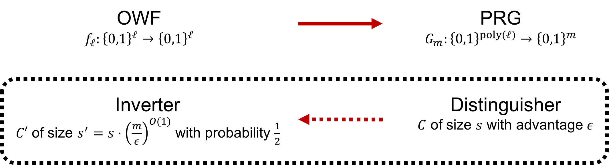
As a result, if $s’\leq\poly(\ell)$, then $C’$ contradicts to the definition of OWF and thus both $C$ and $C’$ does not exists. That is, $G_m$ is $(t,\epsilon)$-pseudorandom.
Let’s see what kind of complexity-theoretic results we can get from the above theorem.
- Cryptographic OWFs implies $\BPP\subseteq\SUBEXP$.
- Factoring OWF implies $\BPP\subseteq\QP$.
Suppose the OWF is hard to invert by algorithms of running time less than $t(\ell)$. Take $m=1/\epsilon=t(\ell)^{o(1)}$ (i.e., $t(\ell)=m^{\omega(1)}$) and $s=\poly(m)$, we have $s’=O(s\cdot(m/\epsilon)^{O(1)})\leq t(\ell)$ for large enough $\ell$, i.e., contradiction. Thus, $G_m$ is $(\poly(m),1/m)$-pseudorandom with seed length $d=\poly(\ell)=\poly(t^{-1}(m^{\omega(1)}))$.
-
If OWF is hard to invert by super-polynomial time algorithms, i.e., $t(\ell)=\ell^{\omega(1)}$, then $\ell=\poly(m)$ and thus $d=m^{\epsilon}$. Namely, $\BPP\in\SUBEXP$.
-
If cryptographic OWF is hard to invert by sub-exponential time algorithms, i.e., $t(\ell)=2^{\ell^{\Omega(1)}}$, then $\ell=\poly\log(m)$ and thus $d=\poly(\log m)$. Namely, $\BPP\in\QP$.
Note that it is impossible to get $d=O(\log m)$ from this setting since $s$ could be arbitrary polynomial by the definition of cryptographic PRG. This totally make sense since we know that the existence of cryptographic PRG with seed length $O(\log m)$ implies something impossible to happen.
Although we cannot get $\BPP=\P$ from cryptographic PRGs, the above approach still has the potential to do so. Concretely, for $\BPP=\P$, we need $d=O(\log m)$ while the state-of-the-art is $\tilde{O}(\ell^3\cdot\log(m/\epsilon)/\log^2s)$ which is $\tilde{O}(\ell^2)$ when we take the maximum possible hardness $t(\ell)=2^{\Omega(\ell)}$. In Vadhan’s book, he formulated this question into the following open problem.
Given an OWF of hardness $t(\ell)$, can we construct a fully explicit $(s,\epsilon)$-PRG with seed length $d=O(\ell)$ where $s=t\cdot(\epsilon/m)^{O(1)}$.
- The harder the OWF can be inverted, the better PRG we can hope for.
Cryptographic PRGs from cryptographic OWPs
When the functions are permutations, we call it one-way permutations (OWPs).
Let $f:\bit^n\rightarrow\bit^n$ be a permutation, we say $f$ is $(S,\epsilon)$-one-way if for any circuit of size at most $S$, \begin{equation} \bbP_{x\in\bit^n}[C(f(x))=x]\leq\epsilon. \end{equation}
Furthermore, we call a family of permutations $\{f_n\}$ a cryptographic one-way permutation (OWP) if for any $n\in\bbN$, $f_n$ is computable in polynomial time and $(S(n),\epsilon(n))=(n^c,1/n^c)$ for any constant $c$ (sometimes denote as $S(n),1/\epsilon(n)=n^{\omega(1)}$).
It turns out that we can construct probabilistic PRGs with arbitrary polynomial stretch from a OWP.
Let $f:\bit^{\ell}\rightarrow\bit^{\ell}$ be a cryptographic OWP and $m=\poly(\ell)$, $(\langle x,r\rangle,\langle f(x),r\rangle,\langle f(f(x)),r\rangle,\dots,\langle f^{(m-1)}(x),r\rangle)$ is a cryptographic PRG.
The proof is based on locally list-decodable code, which will be introduced in another note.
- Cryptographic OWPs implies $\BPP\subseteq\P$.
Some nice properties of PRGs
In this section, we are going to see several nice properties/equivalence of PRGs.
Multi-sample
Let $X,Y$ be two random variables that are $(t,\epsilon)$-indistinguishable for some $t\in\bbN$ and $\epsilon>0$. For any $k\in\bbN$, let $X_1,\dots,X_k$ be i.i.d. copies of $X$ and $Y_1,\dots,Y_k$ be i.i.d. copies of $Y$, then $(X_1,\dots,X_k)$ and $(Y_1,\dots,Y_k)$ are $(t,k\cdot\epsilon)$-indistinguishable.
Let’s prove by contradiction. Suppose there exists a circuit $C$ of size at most $t$ such that $\card{\bbP[C(X_1,\dots,X_k)=1]-\bbP[C(Y_1,\dots,Y_k)]}>k\cdot\epsilon$. We are going to construct a distinguisher of size at most $t$ for $X$ and $Y$.
First, define $k+1$ hybrids of $X$ and $Y$ as follows.
\begin{align}
H_0 &= (X_1,X_2,\dots,X_{m-1},X_k),\\
H_1 &= (X_1,X_2,\dots,X_{m-1},Y_k),\\
&\vdots\\
H_i &= (X_1,X_2,\dots,X_{m-i},Y_{k-i+1},\dots,Y_k),\\
&\vdots\\
H_m &= (Y_1,Y_2,\dots,Y_k).
\end{align}
As $C$ has at least $k\cdot\epsilon$ advantage between $H_0$ and $H_m$, by averaging argument, there exists $i\in[m]$ such that $C$ has at least $\epsilon$ advantage between $H_{i-1}$ and $H_i$. By averaging argument over the $1\text{st},\dots,(i-1)\text{th},(i+1)\text{th},\dots,k\text{th}$ bits, we know that there exists $a_1,\dots,a_{i-1},a_{i+1},\dots,a_k$ such that \begin{equation} \card{\bbP[C(a_1,\dots,a_{i-1},X_i,a_{i+1},\dots,a_k)=1]-\bbP[C(a_1,\dots,a_{i-1},Y_i,a_{i+1},\dots,a_k)=1]}>\epsilon. \end{equation} That is, $C(a_1,\dots,a_{i-1},\cdot,a_{i+1},\dots,a_k)$ is a distinguisher for $X$ and $Y$ of size at most $t$ with advantage more than $\epsilon$, which is a contradiction.
- non-uniform: advice
Next-bit predictability
Let $X=(X_1,\dots,X_m)$ be random variables. We say $X$ is $(t,\epsilon)$-next-bit unpredictable if for any circuits $C$ of size $t$ and for any $i\in[m-1]$, \begin{equation} \mathbb{P}[C(X_1,\dots,X_{i-1})=X_i]<\frac{1}{2}+\epsilon. \end{equation}
The following theorem shows the equivalence of pseudorandomness and next-bit predictability.
Let $X=(X_1,\dots,X_m)$ be $m$ random variables.
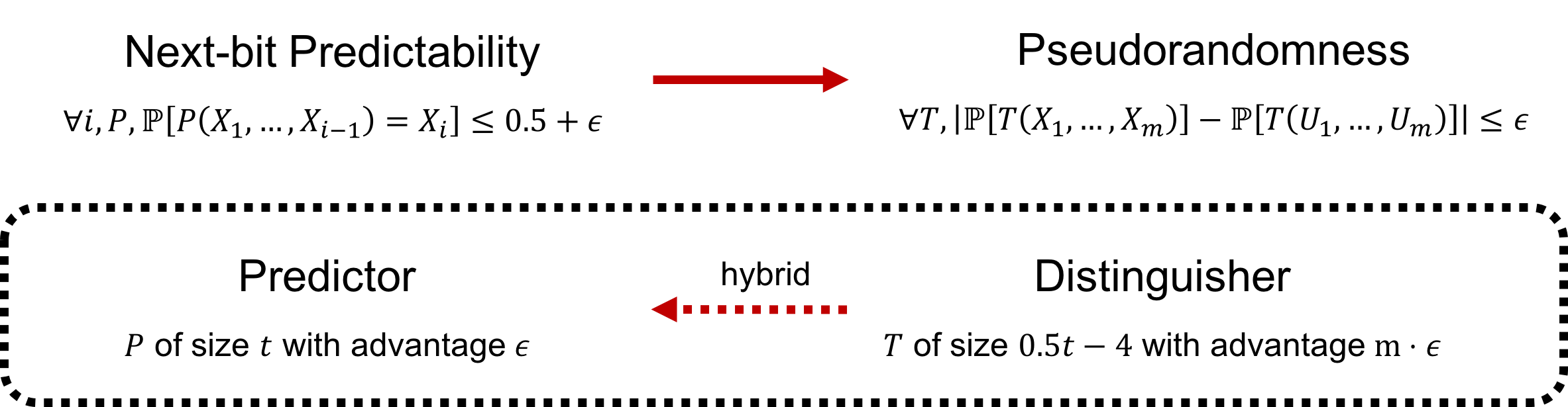
- If $X$ is $(t,\epsilon)$-next-bit unpredictable, then $X$ is $(t/2-4,m\cdot\epsilon)$-pseudorandomness.
- If $X$ is $(t,\epsilon)$-pseudorandom, then $X$ is $(t+3,\epsilon)$-next-bit unpredictable.
- (Next-bit predictability $\Rightarrow$ Pseudorandomness) We are going to show that a distinguisher for $X$ can be transformed into a predictor for $X$.
Suppose $X$ is not $(t/2-4,m\cdot\epsilon)$-pseudorandom. Let $T$ be a distinguisher for $X$ of size $t$ and advantage $\epsilon$. Define $m+1$ hybrids of $X$ as follows.
\begin{align}
H_0 &= (X_1,X_2,\dots,X_{m-1},X_m),\\
H_1 &= (X_1,X_2,\dots,X_{m-1},U_m),\\
&\vdots\\
H_i &= (X_1,X_2,\dots,X_{m-i},U_{m-i+1},\dots,U_m),\\
&\vdots\\
H_m &= (U_1,U_2,\dots,U_m).
\end{align}
As $X$ can be distinguished by $T$ with advantage $\epsilon$, we have
\begin{align}
\card{\bbP[T(H_0)=1]-\bbP[T(U)=1]}>m\cdot\epsilon,
\card{\bbP[T(H_m)=1]-\bbP[T(U)=1]}=0.
\end{align}
That is, $\card{\bbP[T(H_0)=1]-\bbP[T(H-m)=1]}>m\cdot\epsilon$. By the averaging argument, there exists $i\in[m]$ such that
\begin{equation}
\card{\bbP[T(H_{i-1})=1]-\bbP[T(H_i)=1]}>\epsilon.
\end{equation}
Now, we are going to transform $T$ into a predictor $P$ for the $(m-i+1)$th bit of $X$ as follows.
First, by averaging argument, there exists $z_{m-i+2},\dots,z_m$ such that
\begin{align}
&\card{\bbP[T(X_1,\dots,X_{m-i+1},z_{m-i+2},\dots,z_m)=1]\\
-&\bbP[T(X_1,\dots,X_{m-i},U_{m-i+1},z_{m-i+2},\dots,z_m)=1]}>\epsilon.
\end{align}
WLOG, to remove the absolute value operator, assume $\bbP[T(X_1,\dots,X_{m-i+1},z_{m-i+2},\dots,z_m)=1]>\bbP[T(X_1,\dots,X_{m-i},U_{m-i+1},z_{m-i+2},\dots,z_m)=1]$. Next, define the predictor $P$ works as follows. On input $x_1,\dots,x_{m-i}$,
- Compute $T(x_1,\dots,x_{m-i},0)$ and $T(x_1,\dots,x_{m-i},1)$.
- If exactly one of them is 1, then output $b\in\bit$ such that $T(x_1,\dots,x_{m-i},b)=1$.
- Otherwise, randomly output $\bit$.
To construct $P$, one simply needs to compute $T$ twice and do some bit comparison. As we view the randomness as fixed string in nonuniform computational model, $z$ and the randomness used in step 3 will be hard-wired into the circuit. Note that the size of the circuit is at most $2(t/2-4)+8=t$.
To analyze the performance of $P$, define $A=T(X_1,\dots,X_{m-i},X_{m-i+1})$ and $B=T(X_1,\dots,X_{m-i},1-X_{m-i+1})$. By the property of distinguisher $T$, we have
\begin{equation}
\bbP[A=1]>\frac{1}{2}\cdot(\bbP[A=1]+\bbP[B=1])+\epsilon.
\end{equation}
Namely,
\begin{align}
2\epsilon&<\bbP[A=1]-\bbP[B=1]\\
&=\bbP[A=1,B=1]+\bbP[A=1,B=0]-\bbP[A=1,B=1]-\bbP[A=0,B=1]\\
&=\bbP[A=1,B=0]-\bbP[A=0,B=1].
\end{align}
Now, we can compute the predictability of $P$ as follows.
\begin{align}
&\bbP[P(X_1,\dots,X_{m-i})=X_{m-i+1}]\\
&= \frac{1}{2}\cdot\Big(\bbP[A=1,B=1]+\bbP[A=0,B=0]\Big)+\bbP[A=1,B=0]\\
&= \frac{1}{2}\cdot\Big(1-\bbP[A=1,B=0]-\bbP[A=0,B=1]\Big)+\bbP[A=1,B=0]\\
&= \frac{1}{2}+\frac{1}{2}\cdot\Big(\bbP[A=1,B=0]-\bbP[A=0,B=1]\Big)\\
&>\frac{1}{2}+\epsilon.
\end{align}
That is, the existence of a $(t,m\cdot\epsilon)$-distinguisher for $X$ implies a predictor for the $(m-i+1)$th bit of $X$ with advantage $\epsilon$ and size at most $t$.
- (Pseudorandomness $\Rightarrow$ Next-bit predictability) We are going to show that a predictor for $X$ can be transformed into a distinguisher for $X$.
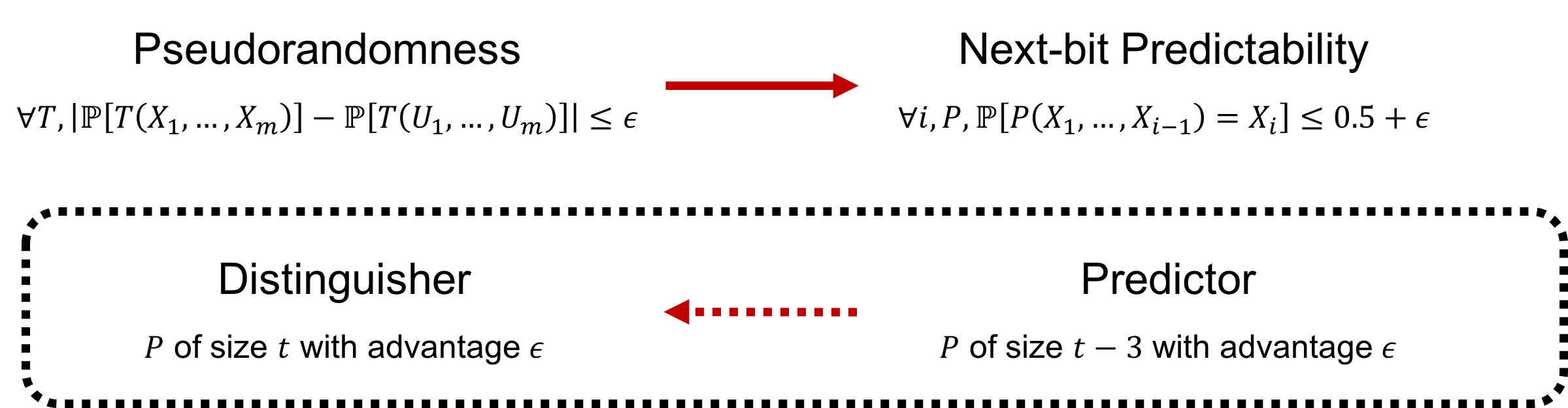
Let $P$ be a $(t-3,\epsilon)$-predictor for the $i$th bit of $X$. Define the distinguisher $T$ as follows. On input $x_1,x_2,\dots,x_m$,
- Compute $P(x_1,\dots,x_{i-1})$.
- If the value is the same as $x_i$, output 1.
- Otherwise, output 0.
Note that the size of $T$ is at most (t-3)+3 since we can construct $T$ explicitly as follows. \begin{equation} T(x_1,\dots,x_m) = (P(x_1,\dots,x_{i-1})\wedge x_i)\vee(\neg P(x_1,\dots,x_{i-1})\wedge\neg x_i). \end{equation}
To verify the distinguishability of $T$, observe that
\begin{align}
\bbP[P(X_1,\dots,X_{i-1})=U_i]&=\frac{1}{2},\\
\bbP[P(X_1,\dots,X_{i-1})=X_i]&>\frac{1}{2}+\epsilon.
\end{align}
Thus, $T$ is a size $t$ $(t,\epsilon)$-distinguisher for $X$.