$
\newcommand{\undefined}{}
\newcommand{\hfill}{}
\newcommand{\qedhere}{\square}
\newcommand{\qed}{\square}
\newcommand{\ensuremath}[1]{#1}
\newcommand{\bit}{\{0,1\}}
\newcommand{\Bit}{\{-1,1\}}
\newcommand{\Stab}{\mathbf{Stab}}
\newcommand{\NS}{\mathbf{NS}}
\newcommand{\ba}{\mathbf{a}}
\newcommand{\bc}{\mathbf{c}}
\newcommand{\bd}{\mathbf{d}}
\newcommand{\be}{\mathbf{e}}
\newcommand{\bh}{\mathbf{h}}
\newcommand{\br}{\mathbf{r}}
\newcommand{\bs}{\mathbf{s}}
\newcommand{\bx}{\mathbf{x}}
\newcommand{\by}{\mathbf{y}}
\newcommand{\bz}{\mathbf{z}}
\newcommand{\Var}{\mathbf{Var}}
\newcommand{\dist}{\text{dist}}
\newcommand{\norm}[1]{\\|#1\\|}
\newcommand{\etal}
\newcommand{\ie}
\newcommand{\eg}
\newcommand{\cf}
\newcommand{\rank}{\text{rank}}
\newcommand{\tr}{\text{tr}}
\newcommand{\mor}{\text{Mor}}
\newcommand{\hom}{\text{Hom}}
\newcommand{\id}{\text{id}}
\newcommand{\obj}{\text{obj}}
\newcommand{\pr}{\text{pr}}
\newcommand{\ker}{\text{ker}}
\newcommand{\coker}{\text{coker}}
\newcommand{\im}{\text{im}}
\newcommand{\vol}{\text{vol}}
\newcommand{\disc}{\text{disc}}
\newcommand{\bbA}{\mathbb A}
\newcommand{\bbB}{\mathbb B}
\newcommand{\bbC}{\mathbb C}
\newcommand{\bbD}{\mathbb D}
\newcommand{\bbE}{\mathbb E}
\newcommand{\bbF}{\mathbb F}
\newcommand{\bbG}{\mathbb G}
\newcommand{\bbH}{\mathbb H}
\newcommand{\bbI}{\mathbb I}
\newcommand{\bbJ}{\mathbb J}
\newcommand{\bbK}{\mathbb K}
\newcommand{\bbL}{\mathbb L}
\newcommand{\bbM}{\mathbb M}
\newcommand{\bbN}{\mathbb N}
\newcommand{\bbO}{\mathbb O}
\newcommand{\bbP}{\mathbb P}
\newcommand{\bbQ}{\mathbb Q}
\newcommand{\bbR}{\mathbb R}
\newcommand{\bbS}{\mathbb S}
\newcommand{\bbT}{\mathbb T}
\newcommand{\bbU}{\mathbb U}
\newcommand{\bbV}{\mathbb V}
\newcommand{\bbW}{\mathbb W}
\newcommand{\bbX}{\mathbb X}
\newcommand{\bbY}{\mathbb Y}
\newcommand{\bbZ}{\mathbb Z}
\newcommand{\sA}{\mathscr A}
\newcommand{\sB}{\mathscr B}
\newcommand{\sC}{\mathscr C}
\newcommand{\sD}{\mathscr D}
\newcommand{\sE}{\mathscr E}
\newcommand{\sF}{\mathscr F}
\newcommand{\sG}{\mathscr G}
\newcommand{\sH}{\mathscr H}
\newcommand{\sI}{\mathscr I}
\newcommand{\sJ}{\mathscr J}
\newcommand{\sK}{\mathscr K}
\newcommand{\sL}{\mathscr L}
\newcommand{\sM}{\mathscr M}
\newcommand{\sN}{\mathscr N}
\newcommand{\sO}{\mathscr O}
\newcommand{\sP}{\mathscr P}
\newcommand{\sQ}{\mathscr Q}
\newcommand{\sR}{\mathscr R}
\newcommand{\sS}{\mathscr S}
\newcommand{\sT}{\mathscr T}
\newcommand{\sU}{\mathscr U}
\newcommand{\sV}{\mathscr V}
\newcommand{\sW}{\mathscr W}
\newcommand{\sX}{\mathscr X}
\newcommand{\sY}{\mathscr Y}
\newcommand{\sZ}{\mathscr Z}
\newcommand{\sfA}{\mathsf A}
\newcommand{\sfB}{\mathsf B}
\newcommand{\sfC}{\mathsf C}
\newcommand{\sfD}{\mathsf D}
\newcommand{\sfE}{\mathsf E}
\newcommand{\sfF}{\mathsf F}
\newcommand{\sfG}{\mathsf G}
\newcommand{\sfH}{\mathsf H}
\newcommand{\sfI}{\mathsf I}
\newcommand{\sfJ}{\mathsf J}
\newcommand{\sfK}{\mathsf K}
\newcommand{\sfL}{\mathsf L}
\newcommand{\sfM}{\mathsf M}
\newcommand{\sfN}{\mathsf N}
\newcommand{\sfO}{\mathsf O}
\newcommand{\sfP}{\mathsf P}
\newcommand{\sfQ}{\mathsf Q}
\newcommand{\sfR}{\mathsf R}
\newcommand{\sfS}{\mathsf S}
\newcommand{\sfT}{\mathsf T}
\newcommand{\sfU}{\mathsf U}
\newcommand{\sfV}{\mathsf V}
\newcommand{\sfW}{\mathsf W}
\newcommand{\sfX}{\mathsf X}
\newcommand{\sfY}{\mathsf Y}
\newcommand{\sfZ}{\mathsf Z}
\newcommand{\cA}{\mathcal A}
\newcommand{\cB}{\mathcal B}
\newcommand{\cC}{\mathcal C}
\newcommand{\cD}{\mathcal D}
\newcommand{\cE}{\mathcal E}
\newcommand{\cF}{\mathcal F}
\newcommand{\cG}{\mathcal G}
\newcommand{\cH}{\mathcal H}
\newcommand{\cI}{\mathcal I}
\newcommand{\cJ}{\mathcal J}
\newcommand{\cK}{\mathcal K}
\newcommand{\cL}{\mathcal L}
\newcommand{\cM}{\mathcal M}
\newcommand{\cN}{\mathcal N}
\newcommand{\cO}{\mathcal O}
\newcommand{\cP}{\mathcal P}
\newcommand{\cQ}{\mathcal Q}
\newcommand{\cR}{\mathcal R}
\newcommand{\cS}{\mathcal S}
\newcommand{\cT}{\mathcal T}
\newcommand{\cU}{\mathcal U}
\newcommand{\cV}{\mathcal V}
\newcommand{\cW}{\mathcal W}
\newcommand{\cX}{\mathcal X}
\newcommand{\cY}{\mathcal Y}
\newcommand{\cZ}{\mathcal Z}
\newcommand{\bfA}{\mathbf A}
\newcommand{\bfB}{\mathbf B}
\newcommand{\bfC}{\mathbf C}
\newcommand{\bfD}{\mathbf D}
\newcommand{\bfE}{\mathbf E}
\newcommand{\bfF}{\mathbf F}
\newcommand{\bfG}{\mathbf G}
\newcommand{\bfH}{\mathbf H}
\newcommand{\bfI}{\mathbf I}
\newcommand{\bfJ}{\mathbf J}
\newcommand{\bfK}{\mathbf K}
\newcommand{\bfL}{\mathbf L}
\newcommand{\bfM}{\mathbf M}
\newcommand{\bfN}{\mathbf N}
\newcommand{\bfO}{\mathbf O}
\newcommand{\bfP}{\mathbf P}
\newcommand{\bfQ}{\mathbf Q}
\newcommand{\bfR}{\mathbf R}
\newcommand{\bfS}{\mathbf S}
\newcommand{\bfT}{\mathbf T}
\newcommand{\bfU}{\mathbf U}
\newcommand{\bfV}{\mathbf V}
\newcommand{\bfW}{\mathbf W}
\newcommand{\bfX}{\mathbf X}
\newcommand{\bfY}{\mathbf Y}
\newcommand{\bfZ}{\mathbf Z}
\newcommand{\rmA}{\mathrm A}
\newcommand{\rmB}{\mathrm B}
\newcommand{\rmC}{\mathrm C}
\newcommand{\rmD}{\mathrm D}
\newcommand{\rmE}{\mathrm E}
\newcommand{\rmF}{\mathrm F}
\newcommand{\rmG}{\mathrm G}
\newcommand{\rmH}{\mathrm H}
\newcommand{\rmI}{\mathrm I}
\newcommand{\rmJ}{\mathrm J}
\newcommand{\rmK}{\mathrm K}
\newcommand{\rmL}{\mathrm L}
\newcommand{\rmM}{\mathrm M}
\newcommand{\rmN}{\mathrm N}
\newcommand{\rmO}{\mathrm O}
\newcommand{\rmP}{\mathrm P}
\newcommand{\rmQ}{\mathrm Q}
\newcommand{\rmR}{\mathrm R}
\newcommand{\rmS}{\mathrm S}
\newcommand{\rmT}{\mathrm T}
\newcommand{\rmU}{\mathrm U}
\newcommand{\rmV}{\mathrm V}
\newcommand{\rmW}{\mathrm W}
\newcommand{\rmX}{\mathrm X}
\newcommand{\rmY}{\mathrm Y}
\newcommand{\rmZ}{\mathrm Z}
\newcommand{\bb}{\mathbf{b}}
\newcommand{\bv}{\mathbf{v}}
\newcommand{\bw}{\mathbf{w}}
\newcommand{\bx}{\mathbf{x}}
\newcommand{\by}{\mathbf{y}}
\newcommand{\bz}{\mathbf{z}}
\newcommand{\paren}[1]{( #1 )}
\newcommand{\Paren}[1]{\left( #1 \right)}
\newcommand{\bigparen}[1]{\bigl( #1 \bigr)}
\newcommand{\Bigparen}[1]{\Bigl( #1 \Bigr)}
\newcommand{\biggparen}[1]{\biggl( #1 \biggr)}
\newcommand{\Biggparen}[1]{\Biggl( #1 \Biggr)}
\newcommand{\abs}[1]{\lvert #1 \rvert}
\newcommand{\Abs}[1]{\left\lvert #1 \right\rvert}
\newcommand{\bigabs}[1]{\bigl\lvert #1 \bigr\rvert}
\newcommand{\Bigabs}[1]{\Bigl\lvert #1 \Bigr\rvert}
\newcommand{\biggabs}[1]{\biggl\lvert #1 \biggr\rvert}
\newcommand{\Biggabs}[1]{\Biggl\lvert #1 \Biggr\rvert}
\newcommand{\card}[1]{\left| #1 \right|}
\newcommand{\Card}[1]{\left\lvert #1 \right\rvert}
\newcommand{\bigcard}[1]{\bigl\lvert #1 \bigr\rvert}
\newcommand{\Bigcard}[1]{\Bigl\lvert #1 \Bigr\rvert}
\newcommand{\biggcard}[1]{\biggl\lvert #1 \biggr\rvert}
\newcommand{\Biggcard}[1]{\Biggl\lvert #1 \Biggr\rvert}
\newcommand{\norm}[1]{\lVert #1 \rVert}
\newcommand{\Norm}[1]{\left\lVert #1 \right\rVert}
\newcommand{\bignorm}[1]{\bigl\lVert #1 \bigr\rVert}
\newcommand{\Bignorm}[1]{\Bigl\lVert #1 \Bigr\rVert}
\newcommand{\biggnorm}[1]{\biggl\lVert #1 \biggr\rVert}
\newcommand{\Biggnorm}[1]{\Biggl\lVert #1 \Biggr\rVert}
\newcommand{\iprod}[1]{\langle #1 \rangle}
\newcommand{\Iprod}[1]{\left\langle #1 \right\rangle}
\newcommand{\bigiprod}[1]{\bigl\langle #1 \bigr\rangle}
\newcommand{\Bigiprod}[1]{\Bigl\langle #1 \Bigr\rangle}
\newcommand{\biggiprod}[1]{\biggl\langle #1 \biggr\rangle}
\newcommand{\Biggiprod}[1]{\Biggl\langle #1 \Biggr\rangle}
\newcommand{\set}[1]{\lbrace #1 \rbrace}
\newcommand{\Set}[1]{\left\lbrace #1 \right\rbrace}
\newcommand{\bigset}[1]{\bigl\lbrace #1 \bigr\rbrace}
\newcommand{\Bigset}[1]{\Bigl\lbrace #1 \Bigr\rbrace}
\newcommand{\biggset}[1]{\biggl\lbrace #1 \biggr\rbrace}
\newcommand{\Biggset}[1]{\Biggl\lbrace #1 \Biggr\rbrace}
\newcommand{\bracket}[1]{\lbrack #1 \rbrack}
\newcommand{\Bracket}[1]{\left\lbrack #1 \right\rbrack}
\newcommand{\bigbracket}[1]{\bigl\lbrack #1 \bigr\rbrack}
\newcommand{\Bigbracket}[1]{\Bigl\lbrack #1 \Bigr\rbrack}
\newcommand{\biggbracket}[1]{\biggl\lbrack #1 \biggr\rbrack}
\newcommand{\Biggbracket}[1]{\Biggl\lbrack #1 \Biggr\rbrack}
\newcommand{\ucorner}[1]{\ulcorner #1 \urcorner}
\newcommand{\Ucorner}[1]{\left\ulcorner #1 \right\urcorner}
\newcommand{\bigucorner}[1]{\bigl\ulcorner #1 \bigr\urcorner}
\newcommand{\Bigucorner}[1]{\Bigl\ulcorner #1 \Bigr\urcorner}
\newcommand{\biggucorner}[1]{\biggl\ulcorner #1 \biggr\urcorner}
\newcommand{\Biggucorner}[1]{\Biggl\ulcorner #1 \Biggr\urcorner}
\newcommand{\ceil}[1]{\lceil #1 \rceil}
\newcommand{\Ceil}[1]{\left\lceil #1 \right\rceil}
\newcommand{\bigceil}[1]{\bigl\lceil #1 \bigr\rceil}
\newcommand{\Bigceil}[1]{\Bigl\lceil #1 \Bigr\rceil}
\newcommand{\biggceil}[1]{\biggl\lceil #1 \biggr\rceil}
\newcommand{\Biggceil}[1]{\Biggl\lceil #1 \Biggr\rceil}
\newcommand{\floor}[1]{\lfloor #1 \rfloor}
\newcommand{\Floor}[1]{\left\lfloor #1 \right\rfloor}
\newcommand{\bigfloor}[1]{\bigl\lfloor #1 \bigr\rfloor}
\newcommand{\Bigfloor}[1]{\Bigl\lfloor #1 \Bigr\rfloor}
\newcommand{\biggfloor}[1]{\biggl\lfloor #1 \biggr\rfloor}
\newcommand{\Biggfloor}[1]{\Biggl\lfloor #1 \Biggr\rfloor}
\newcommand{\lcorner}[1]{\llcorner #1 \lrcorner}
\newcommand{\Lcorner}[1]{\left\llcorner #1 \right\lrcorner}
\newcommand{\biglcorner}[1]{\bigl\llcorner #1 \bigr\lrcorner}
\newcommand{\Biglcorner}[1]{\Bigl\llcorner #1 \Bigr\lrcorner}
\newcommand{\bigglcorner}[1]{\biggl\llcorner #1 \biggr\lrcorner}
\newcommand{\Bigglcorner}[1]{\Biggl\llcorner #1 \Biggr\lrcorner}
\newcommand{\ket}[1]{| #1 \rangle}
\newcommand{\bra}[1]{\langle #1 |}
\newcommand{\braket}[2]{\langle #1 | #2 \rangle}
\newcommand{\ketbra}[1]{| #1 \rangle\langle #1 |}
\newcommand{\e}{\varepsilon}
\newcommand{\eps}{\varepsilon}
\newcommand{\from}{\colon}
\newcommand{\super}[2]{#1^{(#2)}}
\newcommand{\varsuper}[2]{#1^{\scriptscriptstyle (#2)}}
\newcommand{\tensor}{\otimes}
\newcommand{\eset}{\emptyset}
\newcommand{\sse}{\subseteq}
\newcommand{\sst}{\substack}
\newcommand{\ot}{\otimes}
\newcommand{\Esst}[1]{\bbE_{\substack{#1}}}
\newcommand{\vbig}{\vphantom{\bigoplus}}
\newcommand{\seteq}{\mathrel{\mathop:}=}
\newcommand{\defeq}{\stackrel{\mathrm{def}}=}
\newcommand{\Mid}{\mathrel{}\middle|\mathrel{}}
\newcommand{\Ind}{\mathbf 1}
\newcommand{\bits}{\{0,1\}}
\newcommand{\sbits}{\{\pm 1\}}
\newcommand{\R}{\mathbb R}
\newcommand{\Rnn}{\R_{\ge 0}}
\newcommand{\N}{\mathbb N}
\newcommand{\Z}{\mathbb Z}
\newcommand{\Q}{\mathbb Q}
\newcommand{\C}{\mathbb C}
\newcommand{\A}{\mathbb A}
\newcommand{\Real}{\mathbb R}
\newcommand{\mper}{\,.}
\newcommand{\mcom}{\,,}
\DeclareMathOperator{\Id}{Id}
\DeclareMathOperator{\cone}{cone}
\DeclareMathOperator{\vol}{vol}
\DeclareMathOperator{\val}{val}
\DeclareMathOperator{\opt}{opt}
\DeclareMathOperator{\Opt}{Opt}
\DeclareMathOperator{\Val}{Val}
\DeclareMathOperator{\LP}{LP}
\DeclareMathOperator{\SDP}{SDP}
\DeclareMathOperator{\Tr}{Tr}
\DeclareMathOperator{\Inf}{Inf}
\DeclareMathOperator{\size}{size}
\DeclareMathOperator{\poly}{poly}
\DeclareMathOperator{\polylog}{polylog}
\DeclareMathOperator{\min}{min}
\DeclareMathOperator{\max}{max}
\DeclareMathOperator{\argmax}{arg\,max}
\DeclareMathOperator{\argmin}{arg\,min}
\DeclareMathOperator{\qpoly}{qpoly}
\DeclareMathOperator{\qqpoly}{qqpoly}
\DeclareMathOperator{\conv}{conv}
\DeclareMathOperator{\Conv}{Conv}
\DeclareMathOperator{\supp}{supp}
\DeclareMathOperator{\sign}{sign}
\DeclareMathOperator{\perm}{perm}
\DeclareMathOperator{\mspan}{span}
\DeclareMathOperator{\mrank}{rank}
\DeclareMathOperator{\E}{\mathbb E}
\DeclareMathOperator{\pE}{\tilde{\mathbb E}}
\DeclareMathOperator{\Pr}{\mathbb P}
\DeclareMathOperator{\Span}{Span}
\DeclareMathOperator{\Cone}{Cone}
\DeclareMathOperator{\junta}{junta}
\DeclareMathOperator{\NSS}{NSS}
\DeclareMathOperator{\SA}{SA}
\DeclareMathOperator{\SOS}{SOS}
\DeclareMathOperator{\Stab}{\mathbf Stab}
\DeclareMathOperator{\Det}{\textbf{Det}}
\DeclareMathOperator{\Perm}{\textbf{Perm}}
\DeclareMathOperator{\Sym}{\textbf{Sym}}
\DeclareMathOperator{\Pow}{\textbf{Pow}}
\DeclareMathOperator{\Gal}{\textbf{Gal}}
\DeclareMathOperator{\Aut}{\textbf{Aut}}
\newcommand{\iprod}[1]{\langle #1 \rangle}
\newcommand{\cE}{\mathcal{E}}
\newcommand{\E}{\mathbb{E}}
\newcommand{\pE}{\tilde{\mathbb{E}}}
\newcommand{\N}{\mathbb{N}}
\renewcommand{\P}{\mathcal{P}}
\notag
$
$
\newcommand{\sleq}{\ensuremath{\preceq}}
\newcommand{\sgeq}{\ensuremath{\succeq}}
\newcommand{\diag}{\ensuremath{\mathrm{diag}}}
\newcommand{\support}{\ensuremath{\mathrm{support}}}
\newcommand{\zo}{\ensuremath{\{0,1\}}}
\newcommand{\pmo}{\ensuremath{\{\pm 1\}}}
\newcommand{\uppersos}{\ensuremath{\overline{\mathrm{sos}}}}
\newcommand{\lambdamax}{\ensuremath{\lambda_{\mathrm{max}}}}
\newcommand{\rank}{\ensuremath{\mathrm{rank}}}
\newcommand{\Mslow}{\ensuremath{M_{\mathrm{slow}}}}
\newcommand{\Mfast}{\ensuremath{M_{\mathrm{fast}}}}
\newcommand{\Mdiag}{\ensuremath{M_{\mathrm{diag}}}}
\newcommand{\Mcross}{\ensuremath{M_{\mathrm{cross}}}}
\newcommand{\eqdef}{\ensuremath{ =^{def}}}
\newcommand{\threshold}{\ensuremath{\mathrm{threshold}}}
\newcommand{\vbls}{\ensuremath{\mathrm{vbls}}}
\newcommand{\cons}{\ensuremath{\mathrm{cons}}}
\newcommand{\edges}{\ensuremath{\mathrm{edges}}}
\newcommand{\cl}{\ensuremath{\mathrm{cl}}}
\newcommand{\xor}{\ensuremath{\oplus}}
\newcommand{\1}{\ensuremath{\mathrm{1}}}
\notag
$
$
\newcommand{\transpose}[1]{\ensuremath{#1{}^{\mkern-2mu\intercal}}}
\newcommand{\dyad}[1]{\ensuremath{#1#1{}^{\mkern-2mu\intercal}}}
\newcommand{\nchoose}[1]{\ensuremath}
\newcommand{\generated}[1]{\ensuremath{\langle #1 \rangle}}
\notag
$
$
\newcommand{\eqdef}{\mathbin{\stackrel{\rm def}{=}}}
\newcommand{\R} % real numbers
\newcommand{\N}} % natural numbers
\newcommand{\Z} % integers
\newcommand{\F} % a field
\newcommand{\Q} % the rationals
\newcommand{\C}{\mathbb{C}} % the complexes
\newcommand{\poly}}
\newcommand{\polylog}}
\newcommand{\loglog}}}
\newcommand{\zo}{\{0,1\}}
\newcommand{\suchthat}
\newcommand{\pr}[1]{\Pr\left[#1\right]}
\newcommand{\deffont}{\em}
\newcommand{\getsr}{\mathbin{\stackrel{\mbox{\tiny R}}{\gets}}}
\newcommand{\Exp}{\mathop{\mathrm E}\displaylimits} % expectation
\newcommand{\Var}{\mathop{\mathrm Var}\displaylimits} % variance
\newcommand{\xor}{\oplus}
\newcommand{\GF}{\mathrm{GF}}
\newcommand{\eps}{\varepsilon}
\notag
$
$
\newcommand{\class}[1]{\mathbf{#1}}
\newcommand{\coclass}[1]{\mathbf{co\mbox{-}#1}} % and their complements
\newcommand{\BPP}{\class{BPP}}
\newcommand{\NP}{\class{NP}}
\newcommand{\RP}{\class{RP}}
\newcommand{\coRP}{\coclass{RP}}
\newcommand{\ZPP}{\class{ZPP}}
\newcommand{\BQP}{\class{BQP}}
\newcommand{\FP}{\class{FP}}
\newcommand{\QP}{\class{QuasiP}}
\newcommand{\VF}{\class{VF}}
\newcommand{\VBP}{\class{VBP}}
\newcommand{\VP}{\class{VP}}
\newcommand{\VNP}{\class{VNP}}
\newcommand{\RNC}{\class{RNC}}
\newcommand{\RL}{\class{RL}}
\newcommand{\BPL}{\class{BPL}}
\newcommand{\coRL}{\coclass{RL}}
\newcommand{\IP}{\class{IP}}
\newcommand{\AM}{\class{AM}}
\newcommand{\MA}{\class{MA}}
\newcommand{\QMA}{\class{QMA}}
\newcommand{\SBP}{\class{SBP}}
\newcommand{\coAM}{\class{coAM}}
\newcommand{\coMA}{\class{coMA}}
\renewcommand{\P}{\class{P}}
\newcommand\prBPP{\class{prBPP}}
\newcommand\prRP{\class{prRP}}
\newcommand\prP{\class{prP}}
\newcommand{\Ppoly}{\class{P/poly}}
\newcommand{\NPpoly}{\class{NP/poly}}
\newcommand{\coNPpoly}{\class{coNP/poly}}
\newcommand{\DTIME}{\class{DTIME}}
\newcommand{\TIME}{\class{TIME}}
\newcommand{\SIZE}{\class{SIZE}}
\newcommand{\SPACE}{\class{SPACE}}
\newcommand{\ETIME}{\class{E}}
\newcommand{\BPTIME}{\class{BPTIME}}
\newcommand{\RPTIME}{\class{RPTIME}}
\newcommand{\ZPTIME}{\class{ZPTIME}}
\newcommand{\EXP}{\class{EXP}}
\newcommand{\ZPEXP}{\class{ZPEXP}}
\newcommand{\RPEXP}{\class{RPEXP}}
\newcommand{\BPEXP}{\class{BPEXP}}
\newcommand{\SUBEXP}{\class{SUBEXP}}
\newcommand{\NTIME}{\class{NTIME}}
\newcommand{\NL}{\class{NL}}
\renewcommand{\L}{\class{L}}
\newcommand{\NQP}{\class{NQP}}
\newcommand{\NEXP}{\class{NEXP}}
\newcommand{\coNEXP}{\coclass{NEXP}}
\newcommand{\NPSPACE}{\class{NPSPACE}}
\newcommand{\PSPACE}{\class{PSPACE}}
\newcommand{\NSPACE}{\class{NSPACE}}
\newcommand{\coNSPACE}{\coclass{NSPACE}}
\newcommand{\coL}{\coclass{L}}
\newcommand{\coP}{\coclass{P}}
\newcommand{\coNP}{\coclass{NP}}
\newcommand{\coNL}{\coclass{NL}}
\newcommand{\coNPSPACE}{\coclass{NPSPACE}}
\newcommand{\APSPACE}{\class{APSPACE}}
\newcommand{\LINSPACE}{\class{LINSPACE}}
\newcommand{\qP}{\class{\tilde{P}}}
\newcommand{\PH}{\class{PH}}
\newcommand{\EXPSPACE}{\class{EXPSPACE}}
\newcommand{\SigmaTIME}[1]{\class{\Sigma_{#1}TIME}}
\newcommand{\PiTIME}[1]{\class{\Pi_{#1}TIME}}
\newcommand{\SigmaP}[1]{\class{\Sigma_{#1}P}}
\newcommand{\PiP}[1]{\class{\Pi_{#1}P}}
\newcommand{\DeltaP}[1]{\class{\Delta_{#1}P}}
\newcommand{\ATIME}{\class{ATIME}}
\newcommand{\ASPACE}{\class{ASPACE}}
\newcommand{\AP}{\class{AP}}
\newcommand{\AL}{\class{AL}}
\newcommand{\APSPACE}{\class{APSPACE}}
\newcommand{\VNC}[1]{\class{VNC^{#1}}}
\newcommand{\NC}[1]{\class{NC^{#1}}}
\newcommand{\AC}[1]{\class{AC^{#1}}}
\newcommand{\ACC}[1]{\class{ACC^{#1}}}
\newcommand{\TC}[1]{\class{TC^{#1}}}
\newcommand{\ShP}{\class{\# P}}
\newcommand{\PaP}{\class{\oplus P}}
\newcommand{\PCP}{\class{PCP}}
\newcommand{\kMIP}[1]{\class{#1\mbox{-}MIP}}
\newcommand{\MIP}{\class{MIP}}
$
$
\newcommand{\textprob}[1]{\text{#1}}
\newcommand{\mathprob}[1]{\textbf{#1}}
\newcommand{\Satisfiability}{\textprob{Satisfiability}}
\newcommand{\SAT}{\textprob{SAT}}
\newcommand{\TSAT}{\textprob{3SAT}}
\newcommand{\USAT}{\textprob{USAT}}
\newcommand{\UNSAT}{\textprob{UNSAT}}
\newcommand{\QPSAT}{\textprob{QPSAT}}
\newcommand{\TQBF}{\textprob{TQBF}}
\newcommand{\LinProg}{\textprob{Linear Programming}}
\newcommand{\LP}{\mathprob{LP}}
\newcommand{\Factor}{\textprob{Factoring}}
\newcommand{\CircVal}{\textprob{Circuit Value}}
\newcommand{\CVAL}{\mathprob{CVAL}}
\newcommand{\CircSat}{\textprob{Circuit Satisfiability}}
\newcommand{\CSAT}{\textprob{CSAT}}
\newcommand{\CycleCovers}{\textprob{Cycle Covers}}
\newcommand{\MonCircVal}{\textprob{Monotone Circuit Value}}
\newcommand{\Reachability}{\textprob{Reachability}}
\newcommand{\Unreachability}{\textprob{Unreachability}}
\newcommand{\RCH}{\mathprob{RCH}}
\newcommand{\BddHalt}{\textprob{Bounded Halting}}
\newcommand{\BH}{\mathprob{BH}}
\newcommand{\DiscreteLog}{\textprob{Discrete Log}}
\newcommand{\REE}{\mathprob{REE}}
\newcommand{\QBF}{\mathprob{QBF}}
\newcommand{\MCSP}{\mathprob{MCSP}}
\newcommand{\GGEO}{\mathprob{GGEO}}
\newcommand{\CKTMIN}{\mathprob{CKT-MIN}}
\newcommand{\MINCKT}{\mathprob{MIN-CKT}}
\newcommand{\IdentityTest}{\textprob{Identity Testing}}
\newcommand{\Majority}{\textprob{Majority}}
\newcommand{\CountIndSets}{\textprob{\#Independent Sets}}
\newcommand{\Parity}{\textprob{Parity}}
\newcommand{\Clique}{\textprob{Clique}}
\newcommand{\CountCycles}{\textprob{#Cycles}}
\newcommand{\CountPerfMatchings}{\textprob{\#Perfect Matchings}}
\newcommand{\CountMatchings}{\textprob{\#Matchings}}
\newcommand{\CountMatch}{\mathprob{\#Matchings}}
\newcommand{\ECSAT}{\mathprob{E#SAT}}
\newcommand{\ShSAT}{\mathprob{#SAT}}
\newcommand{\ShTSAT}{\mathprob{#3SAT}}
\newcommand{\HamCycle}{\textprob{Hamiltonian Cycle}}
\newcommand{\Permanent}{\textprob{Permanent}}
\newcommand{\ModPermanent}{\textprob{Modular Permanent}}
\newcommand{\GraphNoniso}{\textprob{Graph Nonisomorphism}}
\newcommand{\GI}{\mathprob{GI}}
\newcommand{\GNI}{\mathprob{GNI}}
\newcommand{\GraphIso}{\textprob{Graph Isomorphism}}
\newcommand{\QuantBoolForm}{\textprob{Quantified Boolean
Formulae}}
\newcommand{\GenGeography}{\textprob{Generalized Geography}}
\newcommand{\MAXTSAT}{\mathprob{Max3SAT}}
\newcommand{\GapMaxTSAT}{\mathprob{GapMax3SAT}}
\newcommand{\ELIN}{\mathprob{E3LIN2}}
\newcommand{\CSP}{\mathprob{CSP}}
\newcommand{\Lin}{\mathprob{Lin}}
\newcommand{\ONE}{\mathbf{ONE}}
\newcommand{\ZERO}{\mathbf{ZERO}}
\newcommand{\yes}
\newcommand{\no}
$
This is Biology
28 Nov 2021
(See here for an English version)
今年波士頓的九月(注:這篇文章起筆於十月初…),沒有延續暑假的熾熱,反倒充滿了秋意。每當傍晚騎車越過查爾斯河的小橋時,迎面而來的冷風,讓人彷彿置身在冰水中游泳般,十分暢快。原本預期楓葉會因此提早來訪,然而十月第一個週末的理論組賞楓健行,意外的沒有被想像中繽紛的色彩包圍,果真理論和現實還是有差距呀!
才剛踏上Mt. Monadnock的白點步道,就和一個新來的博士後熱絡的聊起了CS和Neuroscience的跨領域研究。先是互相約略分享了一下各自正在探索的問題,接著談起生物研究和CS以及物理研究的不同。什麼樣子的生物研究是“接近現實的”?如何評判一個數學理論模型是“合乎生物性(biologically plausible)”的?在我們倆口沫橫飛的激辯過程中,一瞬間,我突然從他的眼中看到了一個是如此明顯,但是我至今才終於意識到一個生物學家和電腦科學家(以及數學家和物理學家)之間的鴻溝:原來雙方在談論biological plausibility時,心中想的是完全不一樣的東西!
身為受到CS訓練出生的一份子,當我們提到biological plausibility時,心中基本上想的不乏是列下好多個“限制條件”,例如神經元之間的連結通常很局部、神經元的活動通常很稀疏等等。接者再用數學語言刻畫這些限制條件,並且開始一連串的抽象理論推導或電腦模擬分析。然而對生物學家來說,biological plausibility其實並不見得是這麼具體的條列檢查項目,而比較像是通過大量的閱讀和討論後,建構出一個自己以及領域內的世界觀。生物實驗實在充滿太多雜訊以及特例,基本上不可能列出嚴謹的數學條件逐一客觀的檢查,也因此會產生一些很有趣的現象:生物學家有時候反而會沒有電腦科學家想像的如此biologically plausible!
跨領域的研究充滿了挑戰,除了要學習大量其他領域的知識,我覺得最困難的是如何理解和欣賞其他領域的美。在今年暑假前偶然在Facebook上看到朋友推薦了演化生物學大佬Ernst Mayr在二十多年前寫的This is Biology,讓我終於有機會系統性地一窺生物學家心中的生物學到底是什麼樣貌。
一趟建構生物哲學的雲霄飛車之旅
原本只是打算拉著做演化生物學研究的室友一起讀This is Biology,想和他討論以及聽聽他專業的見解,結果他很熱心的組織了一個讀書會,邀請了幾個來自不同領域的朋友,開始了這段建構我的生物哲學的雲霄飛車之旅。
之所以稱之為雲霄飛車,是因為我的心境變化在這三個月中不斷受到挑戰與改變,如今列車緩緩進站,帶著重新建構的價值與信念,下了車準備展開下一段旅程。未來在跨領域研究的路上,一定還會在受到許多刺激和成長,趁現在記憶猶新之際,讓我簡單記錄一下This is Biology帶給我的啟蒙與轉變。
生物學中的美與挑戰
之前和一個做物理的朋友聊天時,常聽他開玩笑說生物學就像是集郵一樣,它的美是在大自然中的多樣性及複雜,而生物學家的工作就是搜集紀錄各種新的發現。相比之下,物理和數學似乎更加“深入”地探索了自然及抽象世界中隱藏的對稱與結構之美。言下之意,往往就會有種優劣之分的階級感浮現。確實物理學家中普遍有種自信,認為自己對於世界有更深刻的理解,而生物學相對起來年輕許多,在許多子領域中還留在做實驗搜集資料的階段。但這樣的現況並不代表哪一門學科比較難或是比較簡單,當走到一個領域的前端時,只要保有著對於對知識的好奇、對學問的嚴謹、對品質的堅持,每往前一步都有其無法比較和取代的意義。
從小我在一個很少接觸大自然的環境中長大,在城市的車水馬龍和數理抽象世界的烏托邦之間,我一直以來無法理解和欣賞生物學的美。還記得剛認識室友的時候,一聽到他要花一兩年的時間幫蝴蝶標本拍照,寫程式分析翅膀的顏色和形狀,我實在很難接受這樣也算是“做研究”。為什麼要花這麼多時間在千萬種生物的其中一種上?為什麼每個種類的蝴蝶搜集六隻標本就足夠做統計分析?為什麼可以在如此不明顯的關聯性分析得出任何推論?
的確,如果從物理和數學本位的角度來檢視,生物研究可能登不上“大雅之堂”。但是為何生物學需要跟物理和數學相提並論呢?將這幾門不同的學科直接比較就像是把音樂和繪畫做比較一樣,個人的主觀喜好會影響理性客觀的思辨。追根究底,由於“審美觀”的不同,造成了不同學科之間的誤解甚至歧視。所以就讓我先從我對生物之美的重新認識作為一個開端,放下成見,試著描繪生物世界的審美觀究竟為何。
從集郵到拼圖:多樣性之美、個體之美、實驗之美
生物學之所以被開玩笑地貼上集郵的標籤,不外乎就是因為生物多樣性。世界上已知的次原子粒子有幾百種,而地球上光是蝴蝶就有將近兩萬種。如果更仔細去想何謂不同的生物種類,就會發現連光是如何好好的定義“物種”都已經是一個非常不簡單的工作了。既然生物多樣性是如此的瑣碎繁雜,那麼它到底美在什麼地方呢?從表面上看起來,的確就像是集郵一樣辨別和搜集不同的物種,這就是多樣性之美嗎?對我來說,這種”集郵之美“只是生物多樣性中的第一步而已,而生物學家在做的則是要在千千萬萬的物種之間,規約找出背後的規律及異同。
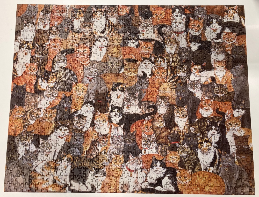
因此我覺得生物的美更多是在於集郵之後的”拼圖“階段。如何在雜亂的實驗數據(i.e., 拼圖碎片)中把有關聯的聚集在一起、如何不受到表面相似性的影響(e.g., 下圖中的貓咪拼圖,同樣是橘色的圖塊,可能是來自於不同的貓咪!)、甚至是如何在缺乏整體圖像(e.g., 想像玩拼圖的時候不讓你看到最後的圖像是什麼)的情況之下,試圖拼湊出些什麼有意義的結果。
至於物理和數學,則比較像是棋盤遊戲和策略遊戲,在少數的規則和龐大的可能性中,堆疊開闢出一條蹊徑。
於是,要建立對生物學的審美觀,需要先暫時放下對從邏輯底層往上前進的堅持,著眼在如何由上而下的把龐大雜亂的資訊梳理乾淨(當然在數理學科也有許多由上而下的美與挑戰,這邊我只是用一個最宏觀的角度來區分生物研究和其不同之處),如果無法欣賞這部分的有趣和美感,那麼可能將會有點困難去進一步體會近代生物研究發展的美。同時在這邊我也想強調,這篇文章的目的不是要說服所有讀者都要能夠欣賞生物之美,而是著重於剖析生物和物理(及數學)本質的差別,然後提出我觀察到不同領域誤解和歧視的癥結點。
當開始可以欣賞生物學中由上而下的“拼圖之美”之後,接下來就會有更多可愛之處可以探索,在這裡我要跟大家分享三個我近期的體悟與感動,分別是多樣性之美、個體之美、實驗之美。
多樣性之美:以前我一直不太能理解每次我室友看到沒見過的螞蟻品種時,為什麼會那麼的興奮(其實現在我也沒有全然理解…)。現在回想起來,最主要是因為過去的我對於美感的追求是更為抽象、型式與對稱,而生物多樣性之美則幾乎是硬幣的另一個反面,欣賞的是具體、實作與特例。兩種美感雖然很不一樣,但是並不互相衝突。因為成長以及學習環境的不同,每個人的確也會對於這兩種美有不同的傾向。當然,一個人不需要強迫自己去欣賞另外一種美,不過當審美的視野被打開了,除了生活增添更多色彩之外,多樣性之美更是時常帶來許多的靈感。
個體之美:每個人在這個世界上都是一個獨一無二的存在,不像是宇宙中的每個氫原子基本上看起來和觀測起來都是一樣的。雖然在前幾段我才說生物學家的工作就是在多樣性中尋找出規律,但也正因為生物世界中的個體總是存在著差異,在發現規律的同時,更是讓我們能夠從個體和規律的偏差之間重新給予其新的理解與認識。生物學中理論的建構,在追尋背後支配現實的規則之餘,可以說是給我們一個新的觀點和角度去理解個體之美。
實驗之美:當物理是要透過精準的實驗驗證理論模型時,我會覺得生物實驗更像是從稀少的資源中試圖以管窺豹。當前面說到我室友的蝴蝶研究中每個物種只用了六隻個體,這並不是說他們不想要用一百隻,而是現實上不允許他們這樣做。於是實驗上的限制(e.g., 蝴蝶的個數、數據中的雜訊)就好比是數學推理中的邏輯規則,生物學家如何在各種限制中設計出有意思的實驗方法,不亞於數學家在邏輯公設中殺出一條血路。差別主要在於這些限制的數量和具體程度,以及邏輯推演的長短。
這邊提供neuroscience中兩個關於decision making的經典實驗,讓讀者體會實驗設計背後的巧思與美感。
首先提供一些背景資訊,在decision making相關的研究中,neuroscientists的(短期)目標是要找到具體的神經網路配置,清楚地對應到一個決策機制。因此最大的挑戰就是該如何盡可能地排除其他可能性,讓實驗結果(只)能被他們提出的理論解釋。於是在一個實驗中,除了各種錄製神經訊號的儀器之外,還需要設計動物行為以及解讀不同的行為結果。
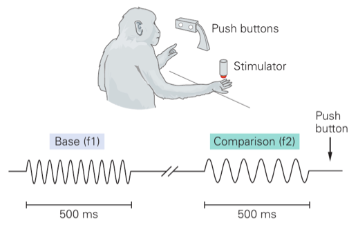
第一個實驗是關於觸覺的decision making。一隻猴子的手指會先被一個20赫茲的震動刺激了500毫秒,再過了一陣了之後,會被另外一個頻率的震動刺激500毫秒。接著猴子必須按鈕決定第二次震動的頻率是比前一次高還是低。
第二個實驗是關於視覺的decision making。一隻猴子首先要盯著一個屏幕上十字,同時看到旁邊有一些小點點全部往左或全部往右移動。最後當十字和小點點同時消失時,猴子必須向右或向左看來表示他覺得小點點大部分是往右還是往左。在比較困難一點的版本,有一部份的小點點會隨機往任何方向移動。
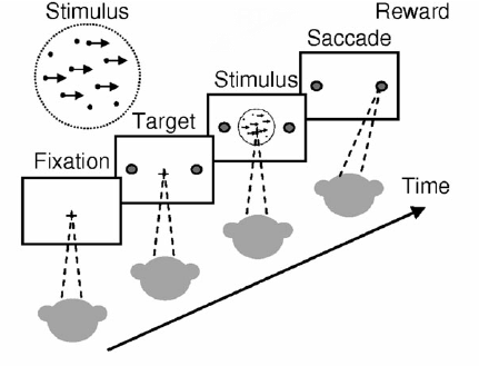
上述這兩個都是非常經典的decision making實驗,但是有沒有其中一個設計得比另一個更為巧妙呢?如果仔細想想的話,就會發現第一個實驗有個很大的問題:兩個震動刺激之間隔了一些時間,因此猴子的大腦需要先“記住”第一個震動,接著再和第二個震動做比較。如此一來增加了可能性的複雜度,而實際上當年的實驗結果也的確無法很好的解釋猴子是如何做決定的。至於第二個實驗,首先透過同時呈現所有資訊來避開了記憶的問題。此外,用不同比例的隨機小點點可以更量化的理解神經網路的機制。先用十字來提醒猴子實驗要開始了更是一個”重新開機“的手法,確保每一次實驗的開端都是差不多的。
不同的挑戰:對稱性的缺乏、湧現性質、客觀意義
如果要再更進一步的建立對生物學的審美觀,就必須正視和理解其面對的挑戰。在這邊我想要著重在三個我個人覺得生物學面臨地最大挑戰:對稱性的缺乏、湧現性質、客觀意義的存在與否。
對稱性的缺乏:近代物理的偉大成就,可以說是建立在對於物理世界中的對稱與不對稱的精闢觀察。對稱性引領出了豐富的數學,使得純粹抽象的分析有了可能(推薦閱讀:The Unreasonable Effectiveness of Mathematics in Physics)。然而在生物的叢林中,極度缺乏豐富多樣的對稱性,這也是我認為建立好的生物理論最困難的根源。於是雖然看似生物領域中有非常多的數學或計算模型,這些模型更像是一種“描述”而不是像基礎物理模型“刻畫”了真實(不過以我對數學模型是“描述”還是“刻畫”的定義,應用物理許多的研究也是屬於前者)。
湧現性質:生物中所謂的湧現性質(emergence property)其實跟物理中的 混沌現象(chaotic phenomenon)基本上是同一個概念:簡單的規則在大量的使用後產生複雜的結果。我個人更喜歡用理論CS的一個概念來思考湧現性質:單一方向性(one-wayness),也就是說正向運算很容易,但是想要逆推回起點是困難的。一個胚胎如何發展成成熟的個體?基因是如何對應到表型(phenotype)?神經元的活動是怎麼形成計算、智能、意識?我認為湧現性質使得機械性的模型與理解變得極為困難,要嘛我們只能得到很粗淺的宏觀統計,要嘛就是模型本身變得極為複雜無法被理解(e.g., 用深度機器學習去建立模型)。同時,物理時常用到的簡約(reduction)方法也因為湧現性質而變得不太可行。我們也許需要一套有別於現有物理與數學的方式來理解湧現性質?
客觀意義:人類總是傾向賦予事物一些意義。還記得上次去羚羊谷(Antelope Canyon))旅行時,除了被大自然的鬼斧神工震撼之外,更是見識了當地導遊的創意。在短短一英哩的路程中,每走幾步導遊就會突然指著岩壁喊著:「看,這是海底總動員裡面的那隻鯊魚!」(如下圖)之類的話。我相信沒有人會覺得大自然是故意侵蝕出一隻鯊魚在羚羊谷裡面,同時這也警惕著我們在面對自然的時候更應該注意放下過多的人為解釋。這不禁讓我想到書裡討論到在過去和近代對於近因與遠因(Proximate and Ultimate cause)不同的觀點,對於一個科學結果的解讀是要非常小心的,尤其是各種因果關係之間的詮釋。在像生物這種尚未公理化的學科中,人們不可避免的必須脫離歸納法(induction)和演繹法(deduction)而使用溯因推理(abductive reasoning)。換句話說,一切的知識是建立的觀察而非邏輯公設,因此不存在所謂的真理,只有最好的解釋。然而“最好的解釋”本身是非常主觀的,話語權尤其會掌握在領域專家手中。話說回到近因與遠因,無論定義為何,根本上兩者都參雜了人的主觀意識。生物中的因果關係以及究極意義,是不是無法達到客觀上的共識?
生物學中的知識、理解、理論是什麼?
前面提到的這些例子和觀點,最終其實只是為了醞釀出Mayr在書中非常前面就想要傳達的概念,那就是生物學需要一套和物理(甚至所謂的傳統科學)不一樣的方法和哲學。還記得在讀書會的前幾週,我總是持著相反的意見,認為Mayr會這樣覺得是因為他懂的物理不夠多。如今,我還是不知道Mayr到底懂不懂物理,不過很肯定的是,我之前對生物的認識實在太淺薄了。
於是在這邊我想要紀錄一下我心境上的轉換,希望能夠帶給非生物背景的人作為一些借鏡,同時也讓生物學家(例如我室友)可以更知道一般受物理和數學訓練的學生通常會有什麼樣子的偏見。
科學哲學:生物學家和物理學家之間的誤解
我在大學的時候學過一些基礎的科學哲學,不外乎就是邏輯實證主義(logical positivism)、Kuhn的典範轉移(paradigm shift)以及Popper的否定論(falsification)。年幼無知的我很理所當然的把這些視為科學的公設,直到現在比較有思辨能力後,在受到This is Biology的啟發才重新發現科學哲學的廣闊與無邊。
Mayr在書中討論科學哲學的段落一開頭就說,這些不同流派的思想基本上都還是以物理學(甚至是理論物理學)為中心,並不見得那麼適用在生物學。而我覺得這之間的區隔,可以用一句演化生物學家Stephen Jay Gould一篇有名文章的標題看出來:『演化是事實和理論(Evolution as fact and theory)』。注意到這邊Gould沒有說演化是真實(reality)或真理(truth),而以我對理論物理的粗淺認識,他們追尋的就恰恰是這兩者,這可以從一本我很喜歡由去年諾貝爾物理學獎得主Roger Penrose寫的書的書名『通往真實的道路(The Road to Reality)』看出來。
[...] facts and theories are different things, not rungs in a hierarchy of increasing certainty. Facts are the world's data. Theories are structures of ideas that explain and interpret facts. Facts do not go away when scientists debate rival theories to explain them. Einstein's theory of gravitation replaced Newton's, but apples did not suspend themselves in mid-air, pending the outcome. [...] Moreover, "fact" does not mean "absolute certainty." The final proofs of logic and mathematics flow deductively from stated premises and achieve certainty only because they are not about the empirical world. [...] In science, "fact" can only mean "confirmed to such a degree that it would be perverse to withhold provisional assent." I suppose that apples might start to rise tomorrow, but the possibility does not merit equal time in physics classrooms.
[...] 事實和理論是不一樣的東西,是無法比較誰比誰更為肯定。事實是這個世界的資料,理論則是解讀事實的一些想法和概念。當科學家在爭論對立的理論哪個比較能解釋某個事實時,事實是並不會跑走或改變。當愛因斯坦的重力論取代了牛頓時,蘋果並沒有因此停在半空中等待結果。 [...] "事實"的意思並不是"絕對的肯定",當一個數學邏輯的證明從起始的假設,演繹地流動到最終的結論時,這樣無瑕的成就完全是因為它不是關於現實的世界。 [...] 在科學中,"事實"只能是代表"被確認到了連反對都看起來像是故意找碴那樣的程度"。蘋果的確有可能在明天就變成往上升起,不過這樣的可能性並不值得讓我們花時間在物理課堂中花時間討論。
Evolution as fact and theory by Stephen Jay Gould.
如果要用更近代一點的科學哲學觀念來剖析其在物理學和生物學的異同,我會說前者更傾向於科學實在論(scientific realism)而後者則是工具主義(instrumentalism)。簡單來說,科學實在論的中心思想是相信”理想理論(ideal theory)”的存在,並且主張科學研究的目標就是要往理想的理論前進。而工具主義則是持相反的意見,認為科學理論是個幫助我們理解和認識世界的工具,應著重於解釋和預測觀測到的現象。
在這邊我極度的省略了對於各種科學哲學流派嚴謹的討論,主要目的只是希望給讀者帶來一個種子,在未來可以自行繼續探索(Stanford的哲學百科全書是個不錯的起點)。同時一個很重要的觀念,科學哲學終究是個幫助我們理清楚科學研究的本質與目標,這既不是終點也沒有確切的答案,每個人都可以有不同的喜好,甚至同一個人對於不同的學科和子領域也可以有不一樣的信念。能夠多理解不一樣的觀點,除了充實自己的思想架構之外,更是能夠在未來與不同領域的人接觸時,更體會對方的思考方式。
數學在生物學中的角色與可能?
身為一個理論電腦科學家以及業餘的數學和理論物理愛好者,還是對數學以及形式上的美有很大的追求(和需求)。然而諸如前面討論到的,種種生物學面對的困難不禁讓人懷疑,數學真的也可以在生物學中達到如在物理學中那樣的成就嗎?最近看了一篇arxiv上的文章“A mathematician’s view of the unreasonable ineffectiveness of mathematics in biology”,作者透過對於著名跨領域到生物的數學家Israel Gelfand的觀察,提出了許多精闢的觀察和故事,蠻值得一個輕鬆的閱讀。
我個人最主要的看法是,現有的數學是很受到物理的影響,許多分枝都是對應到一些相關的物理子領域。相對來講,幾乎沒有什麼新的數學是受到生物啟發誕生的。這並不是說生物缺乏數學的可能性,而是現有的數學也許還不夠,需要有人替生物學創造出新的數學。
而什麼樣子的數學可能適合生物呢?現在生物物理學家或是生物數學家通常使用的是動力系統(dynamical systems)、微分方程(differential equations)或一些控制理論(control theory)、博弈論(game theory),我認為其中非常缺乏了“演算法(algorithm)”的元素。在這邊我指的是更廣義的演算法,像是到了軟體工程的層次,有不同的子程式組成一個巨大的程式。這樣子用演算法/軟體工程的角度來理解生物系統,不但更接近邏輯運算而因此方便人類理解思考,同時也比前述的傳統數學方法更能夠處理特例、複雜的運算。現今的計算生物學(computational biology)可以說就是使用這樣的方法,只不過目前大多還是停留在寫程式跑模擬的階段,還尚未有很乾淨漂亮的數學語言可以做更抽象的分析。
也許一個可能的未來方向是試著如同Turing給了計算(computation)一個完善的數學根基一樣,在一些生物的子領域提出新的數學語言?最近理論電腦科學界的兩位Blum大佬提出了Conscious Turing Machine的概念,似乎就是個將演算法思維應用在接近生物領域的一個好例子?在接下的寒假,我預計要開一個mini-course關於計算在數學、物理和生物之間概念上的異同,希望屆時可以好好思考探索這個方向!
跨領域的現實、包容與理解、下一步
除了This is Biology的讀書會之外,在過去的一年半之間,我和Brabeeba也經營了一個跨領域的讀書會(When neuroscience meets CS, math, and physics),讓我徹底地體會到了跨領域交流的困難是雙向的:除了自己本身需要學習更多、更站在對方角度思考之外,也必須要建立在於對方感興趣展開一段對話。這也讓我覺得,如果長期要做跨領域研究的方向,那麼勢必要先在不同的領域都紮下根基,理解各自的審美觀,累積一定的專業能力,甚至獲得一定程度領域內的認可。換句話說,就是需要在各個領域都達到基本研究生以上的能力吧!
意會到這樣的現實,初期的確令我有點小小沮喪,不過同時也感到非常興奮,非常期待五年十年後自己在各個感興趣的領域種下的種子漸漸冒出枝枒、開花。在這條有趣但充滿挑戰的孤獨之路上,也期許自己勿忘要包容與理解不同學科的多樣性和差異,有耐心和毅力地一步一步走下去。
(感謝Brabeeba Wang和Wei-Ping Chan對於文章的許多好建議!)