$
\newcommand{\undefined}{}
\newcommand{\hfill}{}
\newcommand{\qedhere}{\square}
\newcommand{\qed}{\square}
\newcommand{\ensuremath}[1]{#1}
\newcommand{\bit}{\{0,1\}}
\newcommand{\Bit}{\{-1,1\}}
\newcommand{\Stab}{\mathbf{Stab}}
\newcommand{\NS}{\mathbf{NS}}
\newcommand{\ba}{\mathbf{a}}
\newcommand{\bc}{\mathbf{c}}
\newcommand{\bd}{\mathbf{d}}
\newcommand{\be}{\mathbf{e}}
\newcommand{\bh}{\mathbf{h}}
\newcommand{\br}{\mathbf{r}}
\newcommand{\bs}{\mathbf{s}}
\newcommand{\bx}{\mathbf{x}}
\newcommand{\by}{\mathbf{y}}
\newcommand{\bz}{\mathbf{z}}
\newcommand{\Var}{\mathbf{Var}}
\newcommand{\dist}{\text{dist}}
\newcommand{\norm}[1]{\\|#1\\|}
\newcommand{\etal}
\newcommand{\ie}
\newcommand{\eg}
\newcommand{\cf}
\newcommand{\rank}{\text{rank}}
\newcommand{\tr}{\text{tr}}
\newcommand{\mor}{\text{Mor}}
\newcommand{\hom}{\text{Hom}}
\newcommand{\id}{\text{id}}
\newcommand{\obj}{\text{obj}}
\newcommand{\pr}{\text{pr}}
\newcommand{\ker}{\text{ker}}
\newcommand{\coker}{\text{coker}}
\newcommand{\im}{\text{im}}
\newcommand{\vol}{\text{vol}}
\newcommand{\disc}{\text{disc}}
\newcommand{\bbA}{\mathbb A}
\newcommand{\bbB}{\mathbb B}
\newcommand{\bbC}{\mathbb C}
\newcommand{\bbD}{\mathbb D}
\newcommand{\bbE}{\mathbb E}
\newcommand{\bbF}{\mathbb F}
\newcommand{\bbG}{\mathbb G}
\newcommand{\bbH}{\mathbb H}
\newcommand{\bbI}{\mathbb I}
\newcommand{\bbJ}{\mathbb J}
\newcommand{\bbK}{\mathbb K}
\newcommand{\bbL}{\mathbb L}
\newcommand{\bbM}{\mathbb M}
\newcommand{\bbN}{\mathbb N}
\newcommand{\bbO}{\mathbb O}
\newcommand{\bbP}{\mathbb P}
\newcommand{\bbQ}{\mathbb Q}
\newcommand{\bbR}{\mathbb R}
\newcommand{\bbS}{\mathbb S}
\newcommand{\bbT}{\mathbb T}
\newcommand{\bbU}{\mathbb U}
\newcommand{\bbV}{\mathbb V}
\newcommand{\bbW}{\mathbb W}
\newcommand{\bbX}{\mathbb X}
\newcommand{\bbY}{\mathbb Y}
\newcommand{\bbZ}{\mathbb Z}
\newcommand{\sA}{\mathscr A}
\newcommand{\sB}{\mathscr B}
\newcommand{\sC}{\mathscr C}
\newcommand{\sD}{\mathscr D}
\newcommand{\sE}{\mathscr E}
\newcommand{\sF}{\mathscr F}
\newcommand{\sG}{\mathscr G}
\newcommand{\sH}{\mathscr H}
\newcommand{\sI}{\mathscr I}
\newcommand{\sJ}{\mathscr J}
\newcommand{\sK}{\mathscr K}
\newcommand{\sL}{\mathscr L}
\newcommand{\sM}{\mathscr M}
\newcommand{\sN}{\mathscr N}
\newcommand{\sO}{\mathscr O}
\newcommand{\sP}{\mathscr P}
\newcommand{\sQ}{\mathscr Q}
\newcommand{\sR}{\mathscr R}
\newcommand{\sS}{\mathscr S}
\newcommand{\sT}{\mathscr T}
\newcommand{\sU}{\mathscr U}
\newcommand{\sV}{\mathscr V}
\newcommand{\sW}{\mathscr W}
\newcommand{\sX}{\mathscr X}
\newcommand{\sY}{\mathscr Y}
\newcommand{\sZ}{\mathscr Z}
\newcommand{\sfA}{\mathsf A}
\newcommand{\sfB}{\mathsf B}
\newcommand{\sfC}{\mathsf C}
\newcommand{\sfD}{\mathsf D}
\newcommand{\sfE}{\mathsf E}
\newcommand{\sfF}{\mathsf F}
\newcommand{\sfG}{\mathsf G}
\newcommand{\sfH}{\mathsf H}
\newcommand{\sfI}{\mathsf I}
\newcommand{\sfJ}{\mathsf J}
\newcommand{\sfK}{\mathsf K}
\newcommand{\sfL}{\mathsf L}
\newcommand{\sfM}{\mathsf M}
\newcommand{\sfN}{\mathsf N}
\newcommand{\sfO}{\mathsf O}
\newcommand{\sfP}{\mathsf P}
\newcommand{\sfQ}{\mathsf Q}
\newcommand{\sfR}{\mathsf R}
\newcommand{\sfS}{\mathsf S}
\newcommand{\sfT}{\mathsf T}
\newcommand{\sfU}{\mathsf U}
\newcommand{\sfV}{\mathsf V}
\newcommand{\sfW}{\mathsf W}
\newcommand{\sfX}{\mathsf X}
\newcommand{\sfY}{\mathsf Y}
\newcommand{\sfZ}{\mathsf Z}
\newcommand{\cA}{\mathcal A}
\newcommand{\cB}{\mathcal B}
\newcommand{\cC}{\mathcal C}
\newcommand{\cD}{\mathcal D}
\newcommand{\cE}{\mathcal E}
\newcommand{\cF}{\mathcal F}
\newcommand{\cG}{\mathcal G}
\newcommand{\cH}{\mathcal H}
\newcommand{\cI}{\mathcal I}
\newcommand{\cJ}{\mathcal J}
\newcommand{\cK}{\mathcal K}
\newcommand{\cL}{\mathcal L}
\newcommand{\cM}{\mathcal M}
\newcommand{\cN}{\mathcal N}
\newcommand{\cO}{\mathcal O}
\newcommand{\cP}{\mathcal P}
\newcommand{\cQ}{\mathcal Q}
\newcommand{\cR}{\mathcal R}
\newcommand{\cS}{\mathcal S}
\newcommand{\cT}{\mathcal T}
\newcommand{\cU}{\mathcal U}
\newcommand{\cV}{\mathcal V}
\newcommand{\cW}{\mathcal W}
\newcommand{\cX}{\mathcal X}
\newcommand{\cY}{\mathcal Y}
\newcommand{\cZ}{\mathcal Z}
\newcommand{\bfA}{\mathbf A}
\newcommand{\bfB}{\mathbf B}
\newcommand{\bfC}{\mathbf C}
\newcommand{\bfD}{\mathbf D}
\newcommand{\bfE}{\mathbf E}
\newcommand{\bfF}{\mathbf F}
\newcommand{\bfG}{\mathbf G}
\newcommand{\bfH}{\mathbf H}
\newcommand{\bfI}{\mathbf I}
\newcommand{\bfJ}{\mathbf J}
\newcommand{\bfK}{\mathbf K}
\newcommand{\bfL}{\mathbf L}
\newcommand{\bfM}{\mathbf M}
\newcommand{\bfN}{\mathbf N}
\newcommand{\bfO}{\mathbf O}
\newcommand{\bfP}{\mathbf P}
\newcommand{\bfQ}{\mathbf Q}
\newcommand{\bfR}{\mathbf R}
\newcommand{\bfS}{\mathbf S}
\newcommand{\bfT}{\mathbf T}
\newcommand{\bfU}{\mathbf U}
\newcommand{\bfV}{\mathbf V}
\newcommand{\bfW}{\mathbf W}
\newcommand{\bfX}{\mathbf X}
\newcommand{\bfY}{\mathbf Y}
\newcommand{\bfZ}{\mathbf Z}
\newcommand{\rmA}{\mathrm A}
\newcommand{\rmB}{\mathrm B}
\newcommand{\rmC}{\mathrm C}
\newcommand{\rmD}{\mathrm D}
\newcommand{\rmE}{\mathrm E}
\newcommand{\rmF}{\mathrm F}
\newcommand{\rmG}{\mathrm G}
\newcommand{\rmH}{\mathrm H}
\newcommand{\rmI}{\mathrm I}
\newcommand{\rmJ}{\mathrm J}
\newcommand{\rmK}{\mathrm K}
\newcommand{\rmL}{\mathrm L}
\newcommand{\rmM}{\mathrm M}
\newcommand{\rmN}{\mathrm N}
\newcommand{\rmO}{\mathrm O}
\newcommand{\rmP}{\mathrm P}
\newcommand{\rmQ}{\mathrm Q}
\newcommand{\rmR}{\mathrm R}
\newcommand{\rmS}{\mathrm S}
\newcommand{\rmT}{\mathrm T}
\newcommand{\rmU}{\mathrm U}
\newcommand{\rmV}{\mathrm V}
\newcommand{\rmW}{\mathrm W}
\newcommand{\rmX}{\mathrm X}
\newcommand{\rmY}{\mathrm Y}
\newcommand{\rmZ}{\mathrm Z}
\newcommand{\bb}{\mathbf{b}}
\newcommand{\bv}{\mathbf{v}}
\newcommand{\bw}{\mathbf{w}}
\newcommand{\bx}{\mathbf{x}}
\newcommand{\by}{\mathbf{y}}
\newcommand{\bz}{\mathbf{z}}
\newcommand{\paren}[1]{( #1 )}
\newcommand{\Paren}[1]{\left( #1 \right)}
\newcommand{\bigparen}[1]{\bigl( #1 \bigr)}
\newcommand{\Bigparen}[1]{\Bigl( #1 \Bigr)}
\newcommand{\biggparen}[1]{\biggl( #1 \biggr)}
\newcommand{\Biggparen}[1]{\Biggl( #1 \Biggr)}
\newcommand{\abs}[1]{\lvert #1 \rvert}
\newcommand{\Abs}[1]{\left\lvert #1 \right\rvert}
\newcommand{\bigabs}[1]{\bigl\lvert #1 \bigr\rvert}
\newcommand{\Bigabs}[1]{\Bigl\lvert #1 \Bigr\rvert}
\newcommand{\biggabs}[1]{\biggl\lvert #1 \biggr\rvert}
\newcommand{\Biggabs}[1]{\Biggl\lvert #1 \Biggr\rvert}
\newcommand{\card}[1]{\left| #1 \right|}
\newcommand{\Card}[1]{\left\lvert #1 \right\rvert}
\newcommand{\bigcard}[1]{\bigl\lvert #1 \bigr\rvert}
\newcommand{\Bigcard}[1]{\Bigl\lvert #1 \Bigr\rvert}
\newcommand{\biggcard}[1]{\biggl\lvert #1 \biggr\rvert}
\newcommand{\Biggcard}[1]{\Biggl\lvert #1 \Biggr\rvert}
\newcommand{\norm}[1]{\lVert #1 \rVert}
\newcommand{\Norm}[1]{\left\lVert #1 \right\rVert}
\newcommand{\bignorm}[1]{\bigl\lVert #1 \bigr\rVert}
\newcommand{\Bignorm}[1]{\Bigl\lVert #1 \Bigr\rVert}
\newcommand{\biggnorm}[1]{\biggl\lVert #1 \biggr\rVert}
\newcommand{\Biggnorm}[1]{\Biggl\lVert #1 \Biggr\rVert}
\newcommand{\iprod}[1]{\langle #1 \rangle}
\newcommand{\Iprod}[1]{\left\langle #1 \right\rangle}
\newcommand{\bigiprod}[1]{\bigl\langle #1 \bigr\rangle}
\newcommand{\Bigiprod}[1]{\Bigl\langle #1 \Bigr\rangle}
\newcommand{\biggiprod}[1]{\biggl\langle #1 \biggr\rangle}
\newcommand{\Biggiprod}[1]{\Biggl\langle #1 \Biggr\rangle}
\newcommand{\set}[1]{\lbrace #1 \rbrace}
\newcommand{\Set}[1]{\left\lbrace #1 \right\rbrace}
\newcommand{\bigset}[1]{\bigl\lbrace #1 \bigr\rbrace}
\newcommand{\Bigset}[1]{\Bigl\lbrace #1 \Bigr\rbrace}
\newcommand{\biggset}[1]{\biggl\lbrace #1 \biggr\rbrace}
\newcommand{\Biggset}[1]{\Biggl\lbrace #1 \Biggr\rbrace}
\newcommand{\bracket}[1]{\lbrack #1 \rbrack}
\newcommand{\Bracket}[1]{\left\lbrack #1 \right\rbrack}
\newcommand{\bigbracket}[1]{\bigl\lbrack #1 \bigr\rbrack}
\newcommand{\Bigbracket}[1]{\Bigl\lbrack #1 \Bigr\rbrack}
\newcommand{\biggbracket}[1]{\biggl\lbrack #1 \biggr\rbrack}
\newcommand{\Biggbracket}[1]{\Biggl\lbrack #1 \Biggr\rbrack}
\newcommand{\ucorner}[1]{\ulcorner #1 \urcorner}
\newcommand{\Ucorner}[1]{\left\ulcorner #1 \right\urcorner}
\newcommand{\bigucorner}[1]{\bigl\ulcorner #1 \bigr\urcorner}
\newcommand{\Bigucorner}[1]{\Bigl\ulcorner #1 \Bigr\urcorner}
\newcommand{\biggucorner}[1]{\biggl\ulcorner #1 \biggr\urcorner}
\newcommand{\Biggucorner}[1]{\Biggl\ulcorner #1 \Biggr\urcorner}
\newcommand{\ceil}[1]{\lceil #1 \rceil}
\newcommand{\Ceil}[1]{\left\lceil #1 \right\rceil}
\newcommand{\bigceil}[1]{\bigl\lceil #1 \bigr\rceil}
\newcommand{\Bigceil}[1]{\Bigl\lceil #1 \Bigr\rceil}
\newcommand{\biggceil}[1]{\biggl\lceil #1 \biggr\rceil}
\newcommand{\Biggceil}[1]{\Biggl\lceil #1 \Biggr\rceil}
\newcommand{\floor}[1]{\lfloor #1 \rfloor}
\newcommand{\Floor}[1]{\left\lfloor #1 \right\rfloor}
\newcommand{\bigfloor}[1]{\bigl\lfloor #1 \bigr\rfloor}
\newcommand{\Bigfloor}[1]{\Bigl\lfloor #1 \Bigr\rfloor}
\newcommand{\biggfloor}[1]{\biggl\lfloor #1 \biggr\rfloor}
\newcommand{\Biggfloor}[1]{\Biggl\lfloor #1 \Biggr\rfloor}
\newcommand{\lcorner}[1]{\llcorner #1 \lrcorner}
\newcommand{\Lcorner}[1]{\left\llcorner #1 \right\lrcorner}
\newcommand{\biglcorner}[1]{\bigl\llcorner #1 \bigr\lrcorner}
\newcommand{\Biglcorner}[1]{\Bigl\llcorner #1 \Bigr\lrcorner}
\newcommand{\bigglcorner}[1]{\biggl\llcorner #1 \biggr\lrcorner}
\newcommand{\Bigglcorner}[1]{\Biggl\llcorner #1 \Biggr\lrcorner}
\newcommand{\ket}[1]{| #1 \rangle}
\newcommand{\bra}[1]{\langle #1 |}
\newcommand{\braket}[2]{\langle #1 | #2 \rangle}
\newcommand{\ketbra}[1]{| #1 \rangle\langle #1 |}
\newcommand{\e}{\varepsilon}
\newcommand{\eps}{\varepsilon}
\newcommand{\from}{\colon}
\newcommand{\super}[2]{#1^{(#2)}}
\newcommand{\varsuper}[2]{#1^{\scriptscriptstyle (#2)}}
\newcommand{\tensor}{\otimes}
\newcommand{\eset}{\emptyset}
\newcommand{\sse}{\subseteq}
\newcommand{\sst}{\substack}
\newcommand{\ot}{\otimes}
\newcommand{\Esst}[1]{\bbE_{\substack{#1}}}
\newcommand{\vbig}{\vphantom{\bigoplus}}
\newcommand{\seteq}{\mathrel{\mathop:}=}
\newcommand{\defeq}{\stackrel{\mathrm{def}}=}
\newcommand{\Mid}{\mathrel{}\middle|\mathrel{}}
\newcommand{\Ind}{\mathbf 1}
\newcommand{\bits}{\{0,1\}}
\newcommand{\sbits}{\{\pm 1\}}
\newcommand{\R}{\mathbb R}
\newcommand{\Rnn}{\R_{\ge 0}}
\newcommand{\N}{\mathbb N}
\newcommand{\Z}{\mathbb Z}
\newcommand{\Q}{\mathbb Q}
\newcommand{\C}{\mathbb C}
\newcommand{\A}{\mathbb A}
\newcommand{\Real}{\mathbb R}
\newcommand{\mper}{\,.}
\newcommand{\mcom}{\,,}
\DeclareMathOperator{\Id}{Id}
\DeclareMathOperator{\cone}{cone}
\DeclareMathOperator{\vol}{vol}
\DeclareMathOperator{\val}{val}
\DeclareMathOperator{\opt}{opt}
\DeclareMathOperator{\Opt}{Opt}
\DeclareMathOperator{\Val}{Val}
\DeclareMathOperator{\LP}{LP}
\DeclareMathOperator{\SDP}{SDP}
\DeclareMathOperator{\Tr}{Tr}
\DeclareMathOperator{\Inf}{Inf}
\DeclareMathOperator{\size}{size}
\DeclareMathOperator{\poly}{poly}
\DeclareMathOperator{\polylog}{polylog}
\DeclareMathOperator{\min}{min}
\DeclareMathOperator{\max}{max}
\DeclareMathOperator{\argmax}{arg\,max}
\DeclareMathOperator{\argmin}{arg\,min}
\DeclareMathOperator{\qpoly}{qpoly}
\DeclareMathOperator{\qqpoly}{qqpoly}
\DeclareMathOperator{\conv}{conv}
\DeclareMathOperator{\Conv}{Conv}
\DeclareMathOperator{\supp}{supp}
\DeclareMathOperator{\sign}{sign}
\DeclareMathOperator{\perm}{perm}
\DeclareMathOperator{\mspan}{span}
\DeclareMathOperator{\mrank}{rank}
\DeclareMathOperator{\E}{\mathbb E}
\DeclareMathOperator{\pE}{\tilde{\mathbb E}}
\DeclareMathOperator{\Pr}{\mathbb P}
\DeclareMathOperator{\Span}{Span}
\DeclareMathOperator{\Cone}{Cone}
\DeclareMathOperator{\junta}{junta}
\DeclareMathOperator{\NSS}{NSS}
\DeclareMathOperator{\SA}{SA}
\DeclareMathOperator{\SOS}{SOS}
\DeclareMathOperator{\Stab}{\mathbf Stab}
\DeclareMathOperator{\Det}{\textbf{Det}}
\DeclareMathOperator{\Perm}{\textbf{Perm}}
\DeclareMathOperator{\Sym}{\textbf{Sym}}
\DeclareMathOperator{\Pow}{\textbf{Pow}}
\DeclareMathOperator{\Gal}{\textbf{Gal}}
\DeclareMathOperator{\Aut}{\textbf{Aut}}
\newcommand{\iprod}[1]{\langle #1 \rangle}
\newcommand{\cE}{\mathcal{E}}
\newcommand{\E}{\mathbb{E}}
\newcommand{\pE}{\tilde{\mathbb{E}}}
\newcommand{\N}{\mathbb{N}}
\renewcommand{\P}{\mathcal{P}}
\notag
$
$
\newcommand{\sleq}{\ensuremath{\preceq}}
\newcommand{\sgeq}{\ensuremath{\succeq}}
\newcommand{\diag}{\ensuremath{\mathrm{diag}}}
\newcommand{\support}{\ensuremath{\mathrm{support}}}
\newcommand{\zo}{\ensuremath{\{0,1\}}}
\newcommand{\pmo}{\ensuremath{\{\pm 1\}}}
\newcommand{\uppersos}{\ensuremath{\overline{\mathrm{sos}}}}
\newcommand{\lambdamax}{\ensuremath{\lambda_{\mathrm{max}}}}
\newcommand{\rank}{\ensuremath{\mathrm{rank}}}
\newcommand{\Mslow}{\ensuremath{M_{\mathrm{slow}}}}
\newcommand{\Mfast}{\ensuremath{M_{\mathrm{fast}}}}
\newcommand{\Mdiag}{\ensuremath{M_{\mathrm{diag}}}}
\newcommand{\Mcross}{\ensuremath{M_{\mathrm{cross}}}}
\newcommand{\eqdef}{\ensuremath{ =^{def}}}
\newcommand{\threshold}{\ensuremath{\mathrm{threshold}}}
\newcommand{\vbls}{\ensuremath{\mathrm{vbls}}}
\newcommand{\cons}{\ensuremath{\mathrm{cons}}}
\newcommand{\edges}{\ensuremath{\mathrm{edges}}}
\newcommand{\cl}{\ensuremath{\mathrm{cl}}}
\newcommand{\xor}{\ensuremath{\oplus}}
\newcommand{\1}{\ensuremath{\mathrm{1}}}
\notag
$
$
\newcommand{\transpose}[1]{\ensuremath{#1{}^{\mkern-2mu\intercal}}}
\newcommand{\dyad}[1]{\ensuremath{#1#1{}^{\mkern-2mu\intercal}}}
\newcommand{\nchoose}[1]{\ensuremath}
\newcommand{\generated}[1]{\ensuremath{\langle #1 \rangle}}
\notag
$
$
\newcommand{\eqdef}{\mathbin{\stackrel{\rm def}{=}}}
\newcommand{\R} % real numbers
\newcommand{\N}} % natural numbers
\newcommand{\Z} % integers
\newcommand{\F} % a field
\newcommand{\Q} % the rationals
\newcommand{\C}{\mathbb{C}} % the complexes
\newcommand{\poly}}
\newcommand{\polylog}}
\newcommand{\loglog}}}
\newcommand{\zo}{\{0,1\}}
\newcommand{\suchthat}
\newcommand{\pr}[1]{\Pr\left[#1\right]}
\newcommand{\deffont}{\em}
\newcommand{\getsr}{\mathbin{\stackrel{\mbox{\tiny R}}{\gets}}}
\newcommand{\Exp}{\mathop{\mathrm E}\displaylimits} % expectation
\newcommand{\Var}{\mathop{\mathrm Var}\displaylimits} % variance
\newcommand{\xor}{\oplus}
\newcommand{\GF}{\mathrm{GF}}
\newcommand{\eps}{\varepsilon}
\notag
$
$
\newcommand{\class}[1]{\mathbf{#1}}
\newcommand{\coclass}[1]{\mathbf{co\mbox{-}#1}} % and their complements
\newcommand{\BPP}{\class{BPP}}
\newcommand{\NP}{\class{NP}}
\newcommand{\RP}{\class{RP}}
\newcommand{\coRP}{\coclass{RP}}
\newcommand{\ZPP}{\class{ZPP}}
\newcommand{\BQP}{\class{BQP}}
\newcommand{\FP}{\class{FP}}
\newcommand{\QP}{\class{QuasiP}}
\newcommand{\VF}{\class{VF}}
\newcommand{\VBP}{\class{VBP}}
\newcommand{\VP}{\class{VP}}
\newcommand{\VNP}{\class{VNP}}
\newcommand{\RNC}{\class{RNC}}
\newcommand{\RL}{\class{RL}}
\newcommand{\BPL}{\class{BPL}}
\newcommand{\coRL}{\coclass{RL}}
\newcommand{\IP}{\class{IP}}
\newcommand{\AM}{\class{AM}}
\newcommand{\MA}{\class{MA}}
\newcommand{\QMA}{\class{QMA}}
\newcommand{\SBP}{\class{SBP}}
\newcommand{\coAM}{\class{coAM}}
\newcommand{\coMA}{\class{coMA}}
\renewcommand{\P}{\class{P}}
\newcommand\prBPP{\class{prBPP}}
\newcommand\prRP{\class{prRP}}
\newcommand\prP{\class{prP}}
\newcommand{\Ppoly}{\class{P/poly}}
\newcommand{\NPpoly}{\class{NP/poly}}
\newcommand{\coNPpoly}{\class{coNP/poly}}
\newcommand{\DTIME}{\class{DTIME}}
\newcommand{\TIME}{\class{TIME}}
\newcommand{\SIZE}{\class{SIZE}}
\newcommand{\SPACE}{\class{SPACE}}
\newcommand{\ETIME}{\class{E}}
\newcommand{\BPTIME}{\class{BPTIME}}
\newcommand{\RPTIME}{\class{RPTIME}}
\newcommand{\ZPTIME}{\class{ZPTIME}}
\newcommand{\EXP}{\class{EXP}}
\newcommand{\ZPEXP}{\class{ZPEXP}}
\newcommand{\RPEXP}{\class{RPEXP}}
\newcommand{\BPEXP}{\class{BPEXP}}
\newcommand{\SUBEXP}{\class{SUBEXP}}
\newcommand{\NTIME}{\class{NTIME}}
\newcommand{\NL}{\class{NL}}
\renewcommand{\L}{\class{L}}
\newcommand{\NQP}{\class{NQP}}
\newcommand{\NEXP}{\class{NEXP}}
\newcommand{\coNEXP}{\coclass{NEXP}}
\newcommand{\NPSPACE}{\class{NPSPACE}}
\newcommand{\PSPACE}{\class{PSPACE}}
\newcommand{\NSPACE}{\class{NSPACE}}
\newcommand{\coNSPACE}{\coclass{NSPACE}}
\newcommand{\coL}{\coclass{L}}
\newcommand{\coP}{\coclass{P}}
\newcommand{\coNP}{\coclass{NP}}
\newcommand{\coNL}{\coclass{NL}}
\newcommand{\coNPSPACE}{\coclass{NPSPACE}}
\newcommand{\APSPACE}{\class{APSPACE}}
\newcommand{\LINSPACE}{\class{LINSPACE}}
\newcommand{\qP}{\class{\tilde{P}}}
\newcommand{\PH}{\class{PH}}
\newcommand{\EXPSPACE}{\class{EXPSPACE}}
\newcommand{\SigmaTIME}[1]{\class{\Sigma_{#1}TIME}}
\newcommand{\PiTIME}[1]{\class{\Pi_{#1}TIME}}
\newcommand{\SigmaP}[1]{\class{\Sigma_{#1}P}}
\newcommand{\PiP}[1]{\class{\Pi_{#1}P}}
\newcommand{\DeltaP}[1]{\class{\Delta_{#1}P}}
\newcommand{\ATIME}{\class{ATIME}}
\newcommand{\ASPACE}{\class{ASPACE}}
\newcommand{\AP}{\class{AP}}
\newcommand{\AL}{\class{AL}}
\newcommand{\APSPACE}{\class{APSPACE}}
\newcommand{\VNC}[1]{\class{VNC^{#1}}}
\newcommand{\NC}[1]{\class{NC^{#1}}}
\newcommand{\AC}[1]{\class{AC^{#1}}}
\newcommand{\ACC}[1]{\class{ACC^{#1}}}
\newcommand{\TC}[1]{\class{TC^{#1}}}
\newcommand{\ShP}{\class{\# P}}
\newcommand{\PaP}{\class{\oplus P}}
\newcommand{\PCP}{\class{PCP}}
\newcommand{\kMIP}[1]{\class{#1\mbox{-}MIP}}
\newcommand{\MIP}{\class{MIP}}
$
$
\newcommand{\textprob}[1]{\text{#1}}
\newcommand{\mathprob}[1]{\textbf{#1}}
\newcommand{\Satisfiability}{\textprob{Satisfiability}}
\newcommand{\SAT}{\textprob{SAT}}
\newcommand{\TSAT}{\textprob{3SAT}}
\newcommand{\USAT}{\textprob{USAT}}
\newcommand{\UNSAT}{\textprob{UNSAT}}
\newcommand{\QPSAT}{\textprob{QPSAT}}
\newcommand{\TQBF}{\textprob{TQBF}}
\newcommand{\LinProg}{\textprob{Linear Programming}}
\newcommand{\LP}{\mathprob{LP}}
\newcommand{\Factor}{\textprob{Factoring}}
\newcommand{\CircVal}{\textprob{Circuit Value}}
\newcommand{\CVAL}{\mathprob{CVAL}}
\newcommand{\CircSat}{\textprob{Circuit Satisfiability}}
\newcommand{\CSAT}{\textprob{CSAT}}
\newcommand{\CycleCovers}{\textprob{Cycle Covers}}
\newcommand{\MonCircVal}{\textprob{Monotone Circuit Value}}
\newcommand{\Reachability}{\textprob{Reachability}}
\newcommand{\Unreachability}{\textprob{Unreachability}}
\newcommand{\RCH}{\mathprob{RCH}}
\newcommand{\BddHalt}{\textprob{Bounded Halting}}
\newcommand{\BH}{\mathprob{BH}}
\newcommand{\DiscreteLog}{\textprob{Discrete Log}}
\newcommand{\REE}{\mathprob{REE}}
\newcommand{\QBF}{\mathprob{QBF}}
\newcommand{\MCSP}{\mathprob{MCSP}}
\newcommand{\GGEO}{\mathprob{GGEO}}
\newcommand{\CKTMIN}{\mathprob{CKT-MIN}}
\newcommand{\MINCKT}{\mathprob{MIN-CKT}}
\newcommand{\IdentityTest}{\textprob{Identity Testing}}
\newcommand{\Majority}{\textprob{Majority}}
\newcommand{\CountIndSets}{\textprob{\#Independent Sets}}
\newcommand{\Parity}{\textprob{Parity}}
\newcommand{\Clique}{\textprob{Clique}}
\newcommand{\CountCycles}{\textprob{#Cycles}}
\newcommand{\CountPerfMatchings}{\textprob{\#Perfect Matchings}}
\newcommand{\CountMatchings}{\textprob{\#Matchings}}
\newcommand{\CountMatch}{\mathprob{\#Matchings}}
\newcommand{\ECSAT}{\mathprob{E#SAT}}
\newcommand{\ShSAT}{\mathprob{#SAT}}
\newcommand{\ShTSAT}{\mathprob{#3SAT}}
\newcommand{\HamCycle}{\textprob{Hamiltonian Cycle}}
\newcommand{\Permanent}{\textprob{Permanent}}
\newcommand{\ModPermanent}{\textprob{Modular Permanent}}
\newcommand{\GraphNoniso}{\textprob{Graph Nonisomorphism}}
\newcommand{\GI}{\mathprob{GI}}
\newcommand{\GNI}{\mathprob{GNI}}
\newcommand{\GraphIso}{\textprob{Graph Isomorphism}}
\newcommand{\QuantBoolForm}{\textprob{Quantified Boolean
Formulae}}
\newcommand{\GenGeography}{\textprob{Generalized Geography}}
\newcommand{\MAXTSAT}{\mathprob{Max3SAT}}
\newcommand{\GapMaxTSAT}{\mathprob{GapMax3SAT}}
\newcommand{\ELIN}{\mathprob{E3LIN2}}
\newcommand{\CSP}{\mathprob{CSP}}
\newcommand{\Lin}{\mathprob{Lin}}
\newcommand{\ONE}{\mathbf{ONE}}
\newcommand{\ZERO}{\mathbf{ZERO}}
\newcommand{\yes}
\newcommand{\no}
$
$
\newcommand{\undefined}{}
\newcommand{\hfill}{}
\newcommand{\qedhere}{\square}
\newcommand{\qed}{\square}
\newcommand{\ensuremath}[1]{#1}
\newcommand{\bit}{\{0,1\}}
\newcommand{\Bit}{\{-1,1\}}
\newcommand{\Stab}{\mathbf{Stab}}
\newcommand{\NS}{\mathbf{NS}}
\newcommand{\ba}{\mathbf{a}}
\newcommand{\bc}{\mathbf{c}}
\newcommand{\bd}{\mathbf{d}}
\newcommand{\be}{\mathbf{e}}
\newcommand{\bh}{\mathbf{h}}
\newcommand{\br}{\mathbf{r}}
\newcommand{\bs}{\mathbf{s}}
\newcommand{\bx}{\mathbf{x}}
\newcommand{\by}{\mathbf{y}}
\newcommand{\bz}{\mathbf{z}}
\newcommand{\Var}{\mathbf{Var}}
\newcommand{\dist}{\text{dist}}
\newcommand{\norm}[1]{\\|#1\\|}
\newcommand{\etal}
\newcommand{\ie}
\newcommand{\eg}
\newcommand{\cf}
\newcommand{\rank}{\text{rank}}
\newcommand{\tr}{\text{tr}}
\newcommand{\mor}{\text{Mor}}
\newcommand{\hom}{\text{Hom}}
\newcommand{\id}{\text{id}}
\newcommand{\obj}{\text{obj}}
\newcommand{\pr}{\text{pr}}
\newcommand{\ker}{\text{ker}}
\newcommand{\coker}{\text{coker}}
\newcommand{\im}{\text{im}}
\newcommand{\vol}{\text{vol}}
\newcommand{\disc}{\text{disc}}
\newcommand{\bbA}{\mathbb A}
\newcommand{\bbB}{\mathbb B}
\newcommand{\bbC}{\mathbb C}
\newcommand{\bbD}{\mathbb D}
\newcommand{\bbE}{\mathbb E}
\newcommand{\bbF}{\mathbb F}
\newcommand{\bbG}{\mathbb G}
\newcommand{\bbH}{\mathbb H}
\newcommand{\bbI}{\mathbb I}
\newcommand{\bbJ}{\mathbb J}
\newcommand{\bbK}{\mathbb K}
\newcommand{\bbL}{\mathbb L}
\newcommand{\bbM}{\mathbb M}
\newcommand{\bbN}{\mathbb N}
\newcommand{\bbO}{\mathbb O}
\newcommand{\bbP}{\mathbb P}
\newcommand{\bbQ}{\mathbb Q}
\newcommand{\bbR}{\mathbb R}
\newcommand{\bbS}{\mathbb S}
\newcommand{\bbT}{\mathbb T}
\newcommand{\bbU}{\mathbb U}
\newcommand{\bbV}{\mathbb V}
\newcommand{\bbW}{\mathbb W}
\newcommand{\bbX}{\mathbb X}
\newcommand{\bbY}{\mathbb Y}
\newcommand{\bbZ}{\mathbb Z}
\newcommand{\sA}{\mathscr A}
\newcommand{\sB}{\mathscr B}
\newcommand{\sC}{\mathscr C}
\newcommand{\sD}{\mathscr D}
\newcommand{\sE}{\mathscr E}
\newcommand{\sF}{\mathscr F}
\newcommand{\sG}{\mathscr G}
\newcommand{\sH}{\mathscr H}
\newcommand{\sI}{\mathscr I}
\newcommand{\sJ}{\mathscr J}
\newcommand{\sK}{\mathscr K}
\newcommand{\sL}{\mathscr L}
\newcommand{\sM}{\mathscr M}
\newcommand{\sN}{\mathscr N}
\newcommand{\sO}{\mathscr O}
\newcommand{\sP}{\mathscr P}
\newcommand{\sQ}{\mathscr Q}
\newcommand{\sR}{\mathscr R}
\newcommand{\sS}{\mathscr S}
\newcommand{\sT}{\mathscr T}
\newcommand{\sU}{\mathscr U}
\newcommand{\sV}{\mathscr V}
\newcommand{\sW}{\mathscr W}
\newcommand{\sX}{\mathscr X}
\newcommand{\sY}{\mathscr Y}
\newcommand{\sZ}{\mathscr Z}
\newcommand{\sfA}{\mathsf A}
\newcommand{\sfB}{\mathsf B}
\newcommand{\sfC}{\mathsf C}
\newcommand{\sfD}{\mathsf D}
\newcommand{\sfE}{\mathsf E}
\newcommand{\sfF}{\mathsf F}
\newcommand{\sfG}{\mathsf G}
\newcommand{\sfH}{\mathsf H}
\newcommand{\sfI}{\mathsf I}
\newcommand{\sfJ}{\mathsf J}
\newcommand{\sfK}{\mathsf K}
\newcommand{\sfL}{\mathsf L}
\newcommand{\sfM}{\mathsf M}
\newcommand{\sfN}{\mathsf N}
\newcommand{\sfO}{\mathsf O}
\newcommand{\sfP}{\mathsf P}
\newcommand{\sfQ}{\mathsf Q}
\newcommand{\sfR}{\mathsf R}
\newcommand{\sfS}{\mathsf S}
\newcommand{\sfT}{\mathsf T}
\newcommand{\sfU}{\mathsf U}
\newcommand{\sfV}{\mathsf V}
\newcommand{\sfW}{\mathsf W}
\newcommand{\sfX}{\mathsf X}
\newcommand{\sfY}{\mathsf Y}
\newcommand{\sfZ}{\mathsf Z}
\newcommand{\cA}{\mathcal A}
\newcommand{\cB}{\mathcal B}
\newcommand{\cC}{\mathcal C}
\newcommand{\cD}{\mathcal D}
\newcommand{\cE}{\mathcal E}
\newcommand{\cF}{\mathcal F}
\newcommand{\cG}{\mathcal G}
\newcommand{\cH}{\mathcal H}
\newcommand{\cI}{\mathcal I}
\newcommand{\cJ}{\mathcal J}
\newcommand{\cK}{\mathcal K}
\newcommand{\cL}{\mathcal L}
\newcommand{\cM}{\mathcal M}
\newcommand{\cN}{\mathcal N}
\newcommand{\cO}{\mathcal O}
\newcommand{\cP}{\mathcal P}
\newcommand{\cQ}{\mathcal Q}
\newcommand{\cR}{\mathcal R}
\newcommand{\cS}{\mathcal S}
\newcommand{\cT}{\mathcal T}
\newcommand{\cU}{\mathcal U}
\newcommand{\cV}{\mathcal V}
\newcommand{\cW}{\mathcal W}
\newcommand{\cX}{\mathcal X}
\newcommand{\cY}{\mathcal Y}
\newcommand{\cZ}{\mathcal Z}
\newcommand{\bfA}{\mathbf A}
\newcommand{\bfB}{\mathbf B}
\newcommand{\bfC}{\mathbf C}
\newcommand{\bfD}{\mathbf D}
\newcommand{\bfE}{\mathbf E}
\newcommand{\bfF}{\mathbf F}
\newcommand{\bfG}{\mathbf G}
\newcommand{\bfH}{\mathbf H}
\newcommand{\bfI}{\mathbf I}
\newcommand{\bfJ}{\mathbf J}
\newcommand{\bfK}{\mathbf K}
\newcommand{\bfL}{\mathbf L}
\newcommand{\bfM}{\mathbf M}
\newcommand{\bfN}{\mathbf N}
\newcommand{\bfO}{\mathbf O}
\newcommand{\bfP}{\mathbf P}
\newcommand{\bfQ}{\mathbf Q}
\newcommand{\bfR}{\mathbf R}
\newcommand{\bfS}{\mathbf S}
\newcommand{\bfT}{\mathbf T}
\newcommand{\bfU}{\mathbf U}
\newcommand{\bfV}{\mathbf V}
\newcommand{\bfW}{\mathbf W}
\newcommand{\bfX}{\mathbf X}
\newcommand{\bfY}{\mathbf Y}
\newcommand{\bfZ}{\mathbf Z}
\newcommand{\rmA}{\mathrm A}
\newcommand{\rmB}{\mathrm B}
\newcommand{\rmC}{\mathrm C}
\newcommand{\rmD}{\mathrm D}
\newcommand{\rmE}{\mathrm E}
\newcommand{\rmF}{\mathrm F}
\newcommand{\rmG}{\mathrm G}
\newcommand{\rmH}{\mathrm H}
\newcommand{\rmI}{\mathrm I}
\newcommand{\rmJ}{\mathrm J}
\newcommand{\rmK}{\mathrm K}
\newcommand{\rmL}{\mathrm L}
\newcommand{\rmM}{\mathrm M}
\newcommand{\rmN}{\mathrm N}
\newcommand{\rmO}{\mathrm O}
\newcommand{\rmP}{\mathrm P}
\newcommand{\rmQ}{\mathrm Q}
\newcommand{\rmR}{\mathrm R}
\newcommand{\rmS}{\mathrm S}
\newcommand{\rmT}{\mathrm T}
\newcommand{\rmU}{\mathrm U}
\newcommand{\rmV}{\mathrm V}
\newcommand{\rmW}{\mathrm W}
\newcommand{\rmX}{\mathrm X}
\newcommand{\rmY}{\mathrm Y}
\newcommand{\rmZ}{\mathrm Z}
\newcommand{\bb}{\mathbf{b}}
\newcommand{\bv}{\mathbf{v}}
\newcommand{\bw}{\mathbf{w}}
\newcommand{\bx}{\mathbf{x}}
\newcommand{\by}{\mathbf{y}}
\newcommand{\bz}{\mathbf{z}}
\newcommand{\paren}[1]{( #1 )}
\newcommand{\Paren}[1]{\left( #1 \right)}
\newcommand{\bigparen}[1]{\bigl( #1 \bigr)}
\newcommand{\Bigparen}[1]{\Bigl( #1 \Bigr)}
\newcommand{\biggparen}[1]{\biggl( #1 \biggr)}
\newcommand{\Biggparen}[1]{\Biggl( #1 \Biggr)}
\newcommand{\abs}[1]{\lvert #1 \rvert}
\newcommand{\Abs}[1]{\left\lvert #1 \right\rvert}
\newcommand{\bigabs}[1]{\bigl\lvert #1 \bigr\rvert}
\newcommand{\Bigabs}[1]{\Bigl\lvert #1 \Bigr\rvert}
\newcommand{\biggabs}[1]{\biggl\lvert #1 \biggr\rvert}
\newcommand{\Biggabs}[1]{\Biggl\lvert #1 \Biggr\rvert}
\newcommand{\card}[1]{\left| #1 \right|}
\newcommand{\Card}[1]{\left\lvert #1 \right\rvert}
\newcommand{\bigcard}[1]{\bigl\lvert #1 \bigr\rvert}
\newcommand{\Bigcard}[1]{\Bigl\lvert #1 \Bigr\rvert}
\newcommand{\biggcard}[1]{\biggl\lvert #1 \biggr\rvert}
\newcommand{\Biggcard}[1]{\Biggl\lvert #1 \Biggr\rvert}
\newcommand{\norm}[1]{\lVert #1 \rVert}
\newcommand{\Norm}[1]{\left\lVert #1 \right\rVert}
\newcommand{\bignorm}[1]{\bigl\lVert #1 \bigr\rVert}
\newcommand{\Bignorm}[1]{\Bigl\lVert #1 \Bigr\rVert}
\newcommand{\biggnorm}[1]{\biggl\lVert #1 \biggr\rVert}
\newcommand{\Biggnorm}[1]{\Biggl\lVert #1 \Biggr\rVert}
\newcommand{\iprod}[1]{\langle #1 \rangle}
\newcommand{\Iprod}[1]{\left\langle #1 \right\rangle}
\newcommand{\bigiprod}[1]{\bigl\langle #1 \bigr\rangle}
\newcommand{\Bigiprod}[1]{\Bigl\langle #1 \Bigr\rangle}
\newcommand{\biggiprod}[1]{\biggl\langle #1 \biggr\rangle}
\newcommand{\Biggiprod}[1]{\Biggl\langle #1 \Biggr\rangle}
\newcommand{\set}[1]{\lbrace #1 \rbrace}
\newcommand{\Set}[1]{\left\lbrace #1 \right\rbrace}
\newcommand{\bigset}[1]{\bigl\lbrace #1 \bigr\rbrace}
\newcommand{\Bigset}[1]{\Bigl\lbrace #1 \Bigr\rbrace}
\newcommand{\biggset}[1]{\biggl\lbrace #1 \biggr\rbrace}
\newcommand{\Biggset}[1]{\Biggl\lbrace #1 \Biggr\rbrace}
\newcommand{\bracket}[1]{\lbrack #1 \rbrack}
\newcommand{\Bracket}[1]{\left\lbrack #1 \right\rbrack}
\newcommand{\bigbracket}[1]{\bigl\lbrack #1 \bigr\rbrack}
\newcommand{\Bigbracket}[1]{\Bigl\lbrack #1 \Bigr\rbrack}
\newcommand{\biggbracket}[1]{\biggl\lbrack #1 \biggr\rbrack}
\newcommand{\Biggbracket}[1]{\Biggl\lbrack #1 \Biggr\rbrack}
\newcommand{\ucorner}[1]{\ulcorner #1 \urcorner}
\newcommand{\Ucorner}[1]{\left\ulcorner #1 \right\urcorner}
\newcommand{\bigucorner}[1]{\bigl\ulcorner #1 \bigr\urcorner}
\newcommand{\Bigucorner}[1]{\Bigl\ulcorner #1 \Bigr\urcorner}
\newcommand{\biggucorner}[1]{\biggl\ulcorner #1 \biggr\urcorner}
\newcommand{\Biggucorner}[1]{\Biggl\ulcorner #1 \Biggr\urcorner}
\newcommand{\ceil}[1]{\lceil #1 \rceil}
\newcommand{\Ceil}[1]{\left\lceil #1 \right\rceil}
\newcommand{\bigceil}[1]{\bigl\lceil #1 \bigr\rceil}
\newcommand{\Bigceil}[1]{\Bigl\lceil #1 \Bigr\rceil}
\newcommand{\biggceil}[1]{\biggl\lceil #1 \biggr\rceil}
\newcommand{\Biggceil}[1]{\Biggl\lceil #1 \Biggr\rceil}
\newcommand{\floor}[1]{\lfloor #1 \rfloor}
\newcommand{\Floor}[1]{\left\lfloor #1 \right\rfloor}
\newcommand{\bigfloor}[1]{\bigl\lfloor #1 \bigr\rfloor}
\newcommand{\Bigfloor}[1]{\Bigl\lfloor #1 \Bigr\rfloor}
\newcommand{\biggfloor}[1]{\biggl\lfloor #1 \biggr\rfloor}
\newcommand{\Biggfloor}[1]{\Biggl\lfloor #1 \Biggr\rfloor}
\newcommand{\lcorner}[1]{\llcorner #1 \lrcorner}
\newcommand{\Lcorner}[1]{\left\llcorner #1 \right\lrcorner}
\newcommand{\biglcorner}[1]{\bigl\llcorner #1 \bigr\lrcorner}
\newcommand{\Biglcorner}[1]{\Bigl\llcorner #1 \Bigr\lrcorner}
\newcommand{\bigglcorner}[1]{\biggl\llcorner #1 \biggr\lrcorner}
\newcommand{\Bigglcorner}[1]{\Biggl\llcorner #1 \Biggr\lrcorner}
\newcommand{\ket}[1]{| #1 \rangle}
\newcommand{\bra}[1]{\langle #1 |}
\newcommand{\braket}[2]{\langle #1 | #2 \rangle}
\newcommand{\ketbra}[1]{| #1 \rangle\langle #1 |}
\newcommand{\e}{\varepsilon}
\newcommand{\eps}{\varepsilon}
\newcommand{\from}{\colon}
\newcommand{\super}[2]{#1^{(#2)}}
\newcommand{\varsuper}[2]{#1^{\scriptscriptstyle (#2)}}
\newcommand{\tensor}{\otimes}
\newcommand{\eset}{\emptyset}
\newcommand{\sse}{\subseteq}
\newcommand{\sst}{\substack}
\newcommand{\ot}{\otimes}
\newcommand{\Esst}[1]{\bbE_{\substack{#1}}}
\newcommand{\vbig}{\vphantom{\bigoplus}}
\newcommand{\seteq}{\mathrel{\mathop:}=}
\newcommand{\defeq}{\stackrel{\mathrm{def}}=}
\newcommand{\Mid}{\mathrel{}\middle|\mathrel{}}
\newcommand{\Ind}{\mathbf 1}
\newcommand{\bits}{\{0,1\}}
\newcommand{\sbits}{\{\pm 1\}}
\newcommand{\R}{\mathbb R}
\newcommand{\Rnn}{\R_{\ge 0}}
\newcommand{\N}{\mathbb N}
\newcommand{\Z}{\mathbb Z}
\newcommand{\Q}{\mathbb Q}
\newcommand{\C}{\mathbb C}
\newcommand{\A}{\mathbb A}
\newcommand{\Real}{\mathbb R}
\newcommand{\mper}{\,.}
\newcommand{\mcom}{\,,}
\DeclareMathOperator{\Id}{Id}
\DeclareMathOperator{\cone}{cone}
\DeclareMathOperator{\vol}{vol}
\DeclareMathOperator{\val}{val}
\DeclareMathOperator{\opt}{opt}
\DeclareMathOperator{\Opt}{Opt}
\DeclareMathOperator{\Val}{Val}
\DeclareMathOperator{\LP}{LP}
\DeclareMathOperator{\SDP}{SDP}
\DeclareMathOperator{\Tr}{Tr}
\DeclareMathOperator{\Inf}{Inf}
\DeclareMathOperator{\size}{size}
\DeclareMathOperator{\poly}{poly}
\DeclareMathOperator{\polylog}{polylog}
\DeclareMathOperator{\min}{min}
\DeclareMathOperator{\max}{max}
\DeclareMathOperator{\argmax}{arg\,max}
\DeclareMathOperator{\argmin}{arg\,min}
\DeclareMathOperator{\qpoly}{qpoly}
\DeclareMathOperator{\qqpoly}{qqpoly}
\DeclareMathOperator{\conv}{conv}
\DeclareMathOperator{\Conv}{Conv}
\DeclareMathOperator{\supp}{supp}
\DeclareMathOperator{\sign}{sign}
\DeclareMathOperator{\perm}{perm}
\DeclareMathOperator{\mspan}{span}
\DeclareMathOperator{\mrank}{rank}
\DeclareMathOperator{\E}{\mathbb E}
\DeclareMathOperator{\pE}{\tilde{\mathbb E}}
\DeclareMathOperator{\Pr}{\mathbb P}
\DeclareMathOperator{\Span}{Span}
\DeclareMathOperator{\Cone}{Cone}
\DeclareMathOperator{\junta}{junta}
\DeclareMathOperator{\NSS}{NSS}
\DeclareMathOperator{\SA}{SA}
\DeclareMathOperator{\SOS}{SOS}
\DeclareMathOperator{\Stab}{\mathbf Stab}
\DeclareMathOperator{\Det}{\textbf{Det}}
\DeclareMathOperator{\Perm}{\textbf{Perm}}
\DeclareMathOperator{\Sym}{\textbf{Sym}}
\DeclareMathOperator{\Pow}{\textbf{Pow}}
\DeclareMathOperator{\Gal}{\textbf{Gal}}
\DeclareMathOperator{\Aut}{\textbf{Aut}}
\newcommand{\iprod}[1]{\langle #1 \rangle}
\newcommand{\cE}{\mathcal{E}}
\newcommand{\E}{\mathbb{E}}
\newcommand{\pE}{\tilde{\mathbb{E}}}
\newcommand{\N}{\mathbb{N}}
\renewcommand{\P}{\mathcal{P}}
\notag
$
$
\newcommand{\sleq}{\ensuremath{\preceq}}
\newcommand{\sgeq}{\ensuremath{\succeq}}
\newcommand{\diag}{\ensuremath{\mathrm{diag}}}
\newcommand{\support}{\ensuremath{\mathrm{support}}}
\newcommand{\zo}{\ensuremath{\{0,1\}}}
\newcommand{\pmo}{\ensuremath{\{\pm 1\}}}
\newcommand{\uppersos}{\ensuremath{\overline{\mathrm{sos}}}}
\newcommand{\lambdamax}{\ensuremath{\lambda_{\mathrm{max}}}}
\newcommand{\rank}{\ensuremath{\mathrm{rank}}}
\newcommand{\Mslow}{\ensuremath{M_{\mathrm{slow}}}}
\newcommand{\Mfast}{\ensuremath{M_{\mathrm{fast}}}}
\newcommand{\Mdiag}{\ensuremath{M_{\mathrm{diag}}}}
\newcommand{\Mcross}{\ensuremath{M_{\mathrm{cross}}}}
\newcommand{\eqdef}{\ensuremath{ =^{def}}}
\newcommand{\threshold}{\ensuremath{\mathrm{threshold}}}
\newcommand{\vbls}{\ensuremath{\mathrm{vbls}}}
\newcommand{\cons}{\ensuremath{\mathrm{cons}}}
\newcommand{\edges}{\ensuremath{\mathrm{edges}}}
\newcommand{\cl}{\ensuremath{\mathrm{cl}}}
\newcommand{\xor}{\ensuremath{\oplus}}
\newcommand{\1}{\ensuremath{\mathrm{1}}}
\notag
$
$
\newcommand{\transpose}[1]{\ensuremath{#1{}^{\mkern-2mu\intercal}}}
\newcommand{\dyad}[1]{\ensuremath{#1#1{}^{\mkern-2mu\intercal}}}
\newcommand{\nchoose}[1]{\ensuremath}
\newcommand{\generated}[1]{\ensuremath{\langle #1 \rangle}}
\notag
$
$
\newcommand{\eqdef}{\mathbin{\stackrel{\rm def}{=}}}
\newcommand{\R} % real numbers
\newcommand{\N}} % natural numbers
\newcommand{\Z} % integers
\newcommand{\F} % a field
\newcommand{\Q} % the rationals
\newcommand{\C}{\mathbb{C}} % the complexes
\newcommand{\poly}}
\newcommand{\polylog}}
\newcommand{\loglog}}}
\newcommand{\zo}{\{0,1\}}
\newcommand{\suchthat}
\newcommand{\pr}[1]{\Pr\left[#1\right]}
\newcommand{\deffont}{\em}
\newcommand{\getsr}{\mathbin{\stackrel{\mbox{\tiny R}}{\gets}}}
\newcommand{\Exp}{\mathop{\mathrm E}\displaylimits} % expectation
\newcommand{\Var}{\mathop{\mathrm Var}\displaylimits} % variance
\newcommand{\xor}{\oplus}
\newcommand{\GF}{\mathrm{GF}}
\newcommand{\eps}{\varepsilon}
\notag
$
$
\newcommand{\class}[1]{\mathbf{#1}}
\newcommand{\coclass}[1]{\mathbf{co\mbox{-}#1}} % and their complements
\newcommand{\BPP}{\class{BPP}}
\newcommand{\NP}{\class{NP}}
\newcommand{\RP}{\class{RP}}
\newcommand{\coRP}{\coclass{RP}}
\newcommand{\ZPP}{\class{ZPP}}
\newcommand{\BQP}{\class{BQP}}
\newcommand{\FP}{\class{FP}}
\newcommand{\QP}{\class{QuasiP}}
\newcommand{\VF}{\class{VF}}
\newcommand{\VBP}{\class{VBP}}
\newcommand{\VP}{\class{VP}}
\newcommand{\VNP}{\class{VNP}}
\newcommand{\RNC}{\class{RNC}}
\newcommand{\RL}{\class{RL}}
\newcommand{\BPL}{\class{BPL}}
\newcommand{\coRL}{\coclass{RL}}
\newcommand{\IP}{\class{IP}}
\newcommand{\AM}{\class{AM}}
\newcommand{\MA}{\class{MA}}
\newcommand{\QMA}{\class{QMA}}
\newcommand{\SBP}{\class{SBP}}
\newcommand{\coAM}{\class{coAM}}
\newcommand{\coMA}{\class{coMA}}
\renewcommand{\P}{\class{P}}
\newcommand\prBPP{\class{prBPP}}
\newcommand\prRP{\class{prRP}}
\newcommand\prP{\class{prP}}
\newcommand{\Ppoly}{\class{P/poly}}
\newcommand{\NPpoly}{\class{NP/poly}}
\newcommand{\coNPpoly}{\class{coNP/poly}}
\newcommand{\DTIME}{\class{DTIME}}
\newcommand{\TIME}{\class{TIME}}
\newcommand{\SIZE}{\class{SIZE}}
\newcommand{\SPACE}{\class{SPACE}}
\newcommand{\ETIME}{\class{E}}
\newcommand{\BPTIME}{\class{BPTIME}}
\newcommand{\RPTIME}{\class{RPTIME}}
\newcommand{\ZPTIME}{\class{ZPTIME}}
\newcommand{\EXP}{\class{EXP}}
\newcommand{\ZPEXP}{\class{ZPEXP}}
\newcommand{\RPEXP}{\class{RPEXP}}
\newcommand{\BPEXP}{\class{BPEXP}}
\newcommand{\SUBEXP}{\class{SUBEXP}}
\newcommand{\NTIME}{\class{NTIME}}
\newcommand{\NL}{\class{NL}}
\renewcommand{\L}{\class{L}}
\newcommand{\NQP}{\class{NQP}}
\newcommand{\NEXP}{\class{NEXP}}
\newcommand{\coNEXP}{\coclass{NEXP}}
\newcommand{\NPSPACE}{\class{NPSPACE}}
\newcommand{\PSPACE}{\class{PSPACE}}
\newcommand{\NSPACE}{\class{NSPACE}}
\newcommand{\coNSPACE}{\coclass{NSPACE}}
\newcommand{\coL}{\coclass{L}}
\newcommand{\coP}{\coclass{P}}
\newcommand{\coNP}{\coclass{NP}}
\newcommand{\coNL}{\coclass{NL}}
\newcommand{\coNPSPACE}{\coclass{NPSPACE}}
\newcommand{\APSPACE}{\class{APSPACE}}
\newcommand{\LINSPACE}{\class{LINSPACE}}
\newcommand{\qP}{\class{\tilde{P}}}
\newcommand{\PH}{\class{PH}}
\newcommand{\EXPSPACE}{\class{EXPSPACE}}
\newcommand{\SigmaTIME}[1]{\class{\Sigma_{#1}TIME}}
\newcommand{\PiTIME}[1]{\class{\Pi_{#1}TIME}}
\newcommand{\SigmaP}[1]{\class{\Sigma_{#1}P}}
\newcommand{\PiP}[1]{\class{\Pi_{#1}P}}
\newcommand{\DeltaP}[1]{\class{\Delta_{#1}P}}
\newcommand{\ATIME}{\class{ATIME}}
\newcommand{\ASPACE}{\class{ASPACE}}
\newcommand{\AP}{\class{AP}}
\newcommand{\AL}{\class{AL}}
\newcommand{\APSPACE}{\class{APSPACE}}
\newcommand{\VNC}[1]{\class{VNC^{#1}}}
\newcommand{\NC}[1]{\class{NC^{#1}}}
\newcommand{\AC}[1]{\class{AC^{#1}}}
\newcommand{\ACC}[1]{\class{ACC^{#1}}}
\newcommand{\TC}[1]{\class{TC^{#1}}}
\newcommand{\ShP}{\class{\# P}}
\newcommand{\PaP}{\class{\oplus P}}
\newcommand{\PCP}{\class{PCP}}
\newcommand{\kMIP}[1]{\class{#1\mbox{-}MIP}}
\newcommand{\MIP}{\class{MIP}}
$
$
\newcommand{\textprob}[1]{\text{#1}}
\newcommand{\mathprob}[1]{\textbf{#1}}
\newcommand{\Satisfiability}{\textprob{Satisfiability}}
\newcommand{\SAT}{\textprob{SAT}}
\newcommand{\TSAT}{\textprob{3SAT}}
\newcommand{\USAT}{\textprob{USAT}}
\newcommand{\UNSAT}{\textprob{UNSAT}}
\newcommand{\QPSAT}{\textprob{QPSAT}}
\newcommand{\TQBF}{\textprob{TQBF}}
\newcommand{\LinProg}{\textprob{Linear Programming}}
\newcommand{\LP}{\mathprob{LP}}
\newcommand{\Factor}{\textprob{Factoring}}
\newcommand{\CircVal}{\textprob{Circuit Value}}
\newcommand{\CVAL}{\mathprob{CVAL}}
\newcommand{\CircSat}{\textprob{Circuit Satisfiability}}
\newcommand{\CSAT}{\textprob{CSAT}}
\newcommand{\CycleCovers}{\textprob{Cycle Covers}}
\newcommand{\MonCircVal}{\textprob{Monotone Circuit Value}}
\newcommand{\Reachability}{\textprob{Reachability}}
\newcommand{\Unreachability}{\textprob{Unreachability}}
\newcommand{\RCH}{\mathprob{RCH}}
\newcommand{\BddHalt}{\textprob{Bounded Halting}}
\newcommand{\BH}{\mathprob{BH}}
\newcommand{\DiscreteLog}{\textprob{Discrete Log}}
\newcommand{\REE}{\mathprob{REE}}
\newcommand{\QBF}{\mathprob{QBF}}
\newcommand{\MCSP}{\mathprob{MCSP}}
\newcommand{\GGEO}{\mathprob{GGEO}}
\newcommand{\CKTMIN}{\mathprob{CKT-MIN}}
\newcommand{\MINCKT}{\mathprob{MIN-CKT}}
\newcommand{\IdentityTest}{\textprob{Identity Testing}}
\newcommand{\Majority}{\textprob{Majority}}
\newcommand{\CountIndSets}{\textprob{\#Independent Sets}}
\newcommand{\Parity}{\textprob{Parity}}
\newcommand{\Clique}{\textprob{Clique}}
\newcommand{\CountCycles}{\textprob{#Cycles}}
\newcommand{\CountPerfMatchings}{\textprob{\#Perfect Matchings}}
\newcommand{\CountMatchings}{\textprob{\#Matchings}}
\newcommand{\CountMatch}{\mathprob{\#Matchings}}
\newcommand{\ECSAT}{\mathprob{E#SAT}}
\newcommand{\ShSAT}{\mathprob{#SAT}}
\newcommand{\ShTSAT}{\mathprob{#3SAT}}
\newcommand{\HamCycle}{\textprob{Hamiltonian Cycle}}
\newcommand{\Permanent}{\textprob{Permanent}}
\newcommand{\ModPermanent}{\textprob{Modular Permanent}}
\newcommand{\GraphNoniso}{\textprob{Graph Nonisomorphism}}
\newcommand{\GI}{\mathprob{GI}}
\newcommand{\GNI}{\mathprob{GNI}}
\newcommand{\GraphIso}{\textprob{Graph Isomorphism}}
\newcommand{\QuantBoolForm}{\textprob{Quantified Boolean
Formulae}}
\newcommand{\GenGeography}{\textprob{Generalized Geography}}
\newcommand{\MAXTSAT}{\mathprob{Max3SAT}}
\newcommand{\GapMaxTSAT}{\mathprob{GapMax3SAT}}
\newcommand{\ELIN}{\mathprob{E3LIN2}}
\newcommand{\CSP}{\mathprob{CSP}}
\newcommand{\Lin}{\mathprob{Lin}}
\newcommand{\ONE}{\mathbf{ONE}}
\newcommand{\ZERO}{\mathbf{ZERO}}
\newcommand{\yes}
\newcommand{\no}
$
A place to record my feeling, my thought, my exploration, and my growth. Since I intend to be casual here so I decided to use Mandarin for most of the posts. I'll translate some of the posts into English on request and put it
02 May 2023
(See here for an English version)
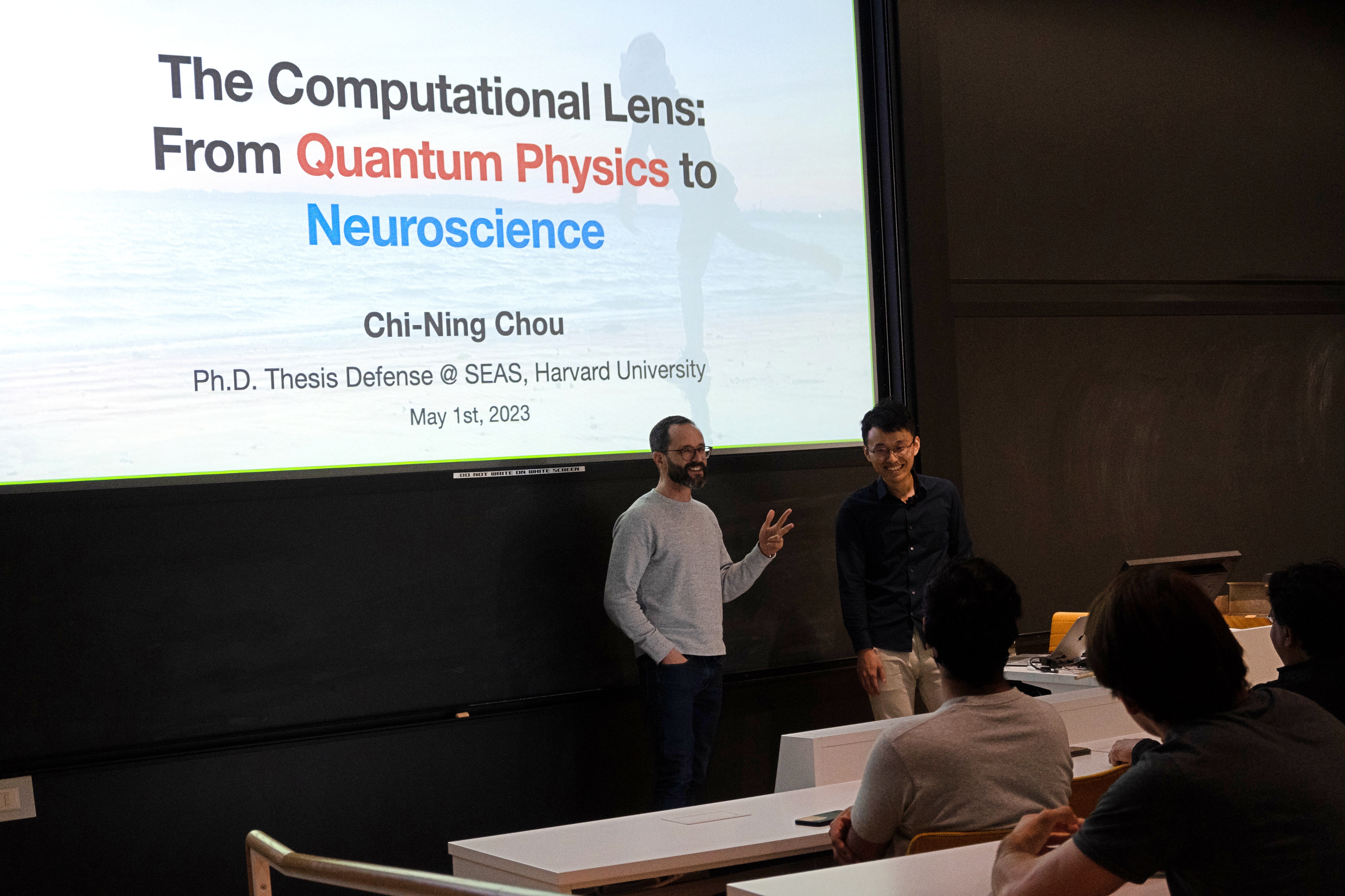
從五六年前就開始想像的那一天,就這樣眨眼間過去了。現在回想起來許多細節仍歷歷在目:一大早烤箱帶來的香氣和悶熱、邊吃著Bagel邊和室友與拜訪的朋友看著跑跑卡丁車敗部復活賽、開車兇猛的Lyft司機、伏地挺身的痠痛。Ph.D.答辯的這一天就像是場籌備已久的舞台劇,一切幾乎都完美地照著劇本走下去(除了洗完澡後從練琴變成了驚喜派對),順暢到連當時的我都沒機會停下來幾秒,閉上眼感受當下心中的悸動。室友跟我說這一天的感覺,大概就跟結婚日差不多。身邊圍繞著這幾年來對我來說很重要的朋友們,我真是個幸福的人。
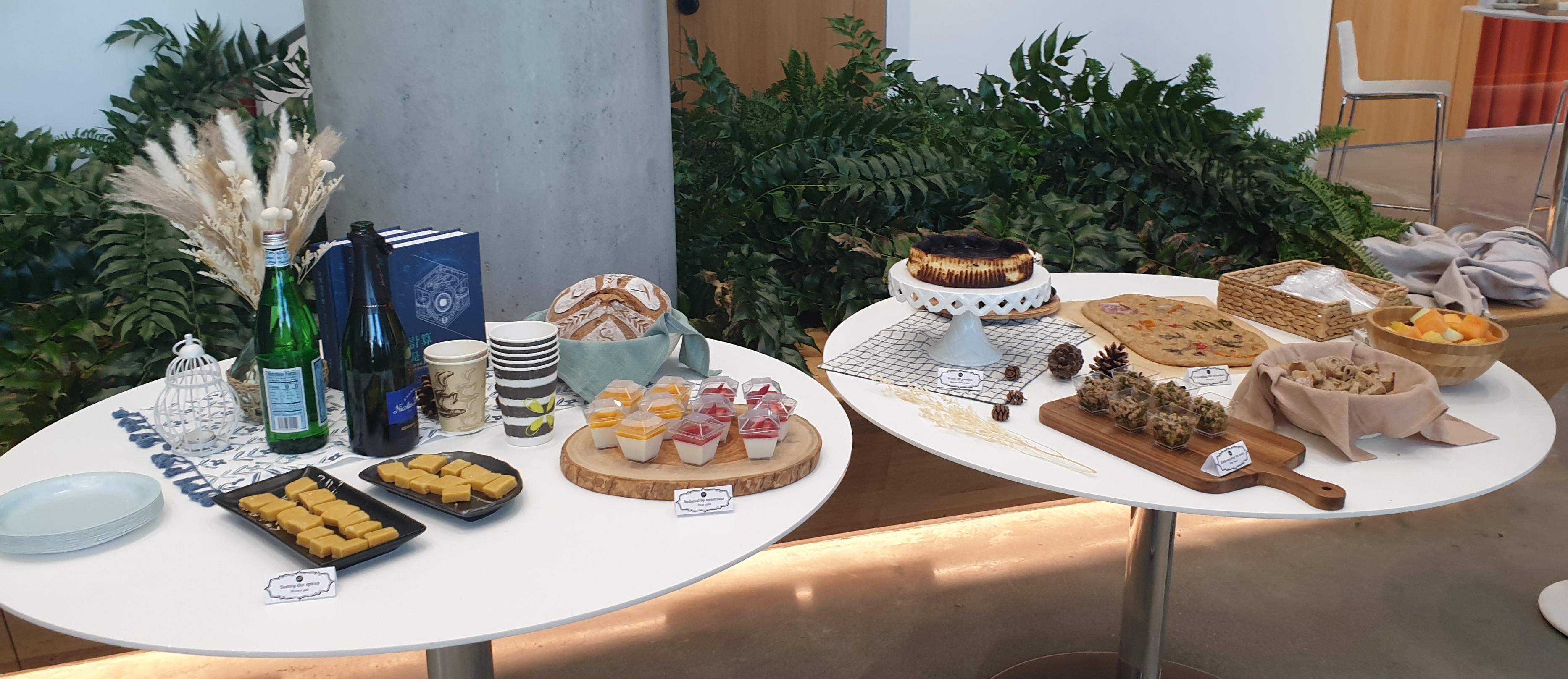
讀博士的這六年,當然是充滿著起起伏伏。在演講後招待會中的六道食物分別暗喻了每一年的心境轉變(感謝大學好友承昌一起想名稱):
初惑甜頭Seduced by sweetness(奶酪):第一年的我就像是個進入甜點店的小孩,看到什麼都想要吃上一口,肆無顧忌地吸取著各種養分。
品香嚐鮮Tasting the spices(Mysore pak):第二年有了許多開會和參加workshop的機會,去了西岸、英國、印度(在那邊嚐到了好吃的Mysore pak)和瑞士,見識到不同的研究風格和環境。
焦心力竭Burnt off passion(巴斯克蛋糕):第三年疫情的襲擊間接地讓我開始重新審視自己做的研究,並對理論CS的方法論產生疑問,對手中研究課題的熱情逐漸消磨。
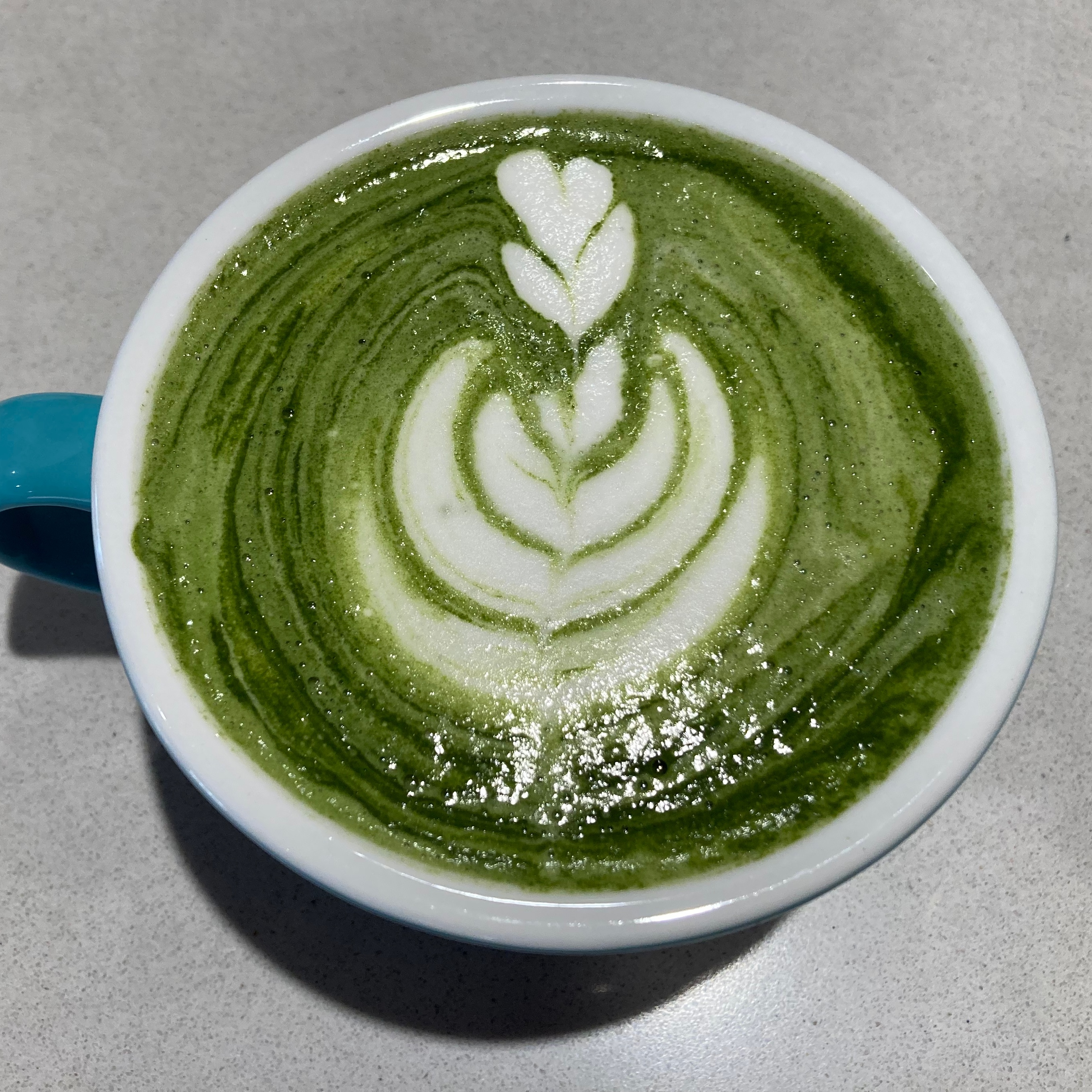
拓邊展界Expanding the boundary(Pizza art):第四年我開始系統性地學習物理和腦神經科學,在研究合作和讀書會中擴展知識的邊界,重新找到對知識追求的熱忱。
揉煉完美Kneading for perfection(Sourdough):第五年我嘗試描繪出未來中長期的研究計畫,完美主義的精神讓我對自己有許多嚴厲的批判,徘徊在不同方法論之間,嘗試找出自己的一條路。
重省初心Rediscovering the roots(蒼蠅頭):第六年時我確定了接下來一步要踏往腦神經科學,同時也漸漸意識到科學方法中必然的不完美,因此漸漸放下對理論CS的批判,重新思考計算能夠扮演的角色。
在傍晚的驚喜派對中,好友L問到我在Ph.D.這幾年有沒有什麼遺憾。當下我很直覺地説,遺憾是一定會有的,就看主觀上我們是如何感受和接納它們。雖然乍聽之下是個故弄玄虛的場面話,但這樣的心態可是近幾年來我慢慢領悟到的道理。我當然很遺憾當年許下的Ph.D.三大目標(拿最佳論文獎、跑波士頓馬拉松、開鋼琴獨奏會)一個都沒有達成,當然很遺憾沒有好好珍惜身邊許多重要的人事物,當然也很遺憾答辯這天錯過了跟好多人講講話、拍照的機會。
但就像棒球教導我的,不管之前被三振了幾次,還是暴傳被教練罵個臭頭。每當站上了球場,過去發生的起起伏伏都是前進的養份,我要讓自己準備好到無論結果如何,都能夠笑著挺胸面對。
時間雖然看似連續地流逝著,但總是讓人在某些時刻能感受到強烈的分野。沈澱了半天後,在雨後前往琴房的途中,依然微涼的晚霞好像看起來不太一樣了。對許多人來說是場再平凡不過的答辯演講,對我來說既是完成了多年的想像,也總結了百轉千折的摸索之路,揭開了人生下一本書的序幕。
17 Sep 2022
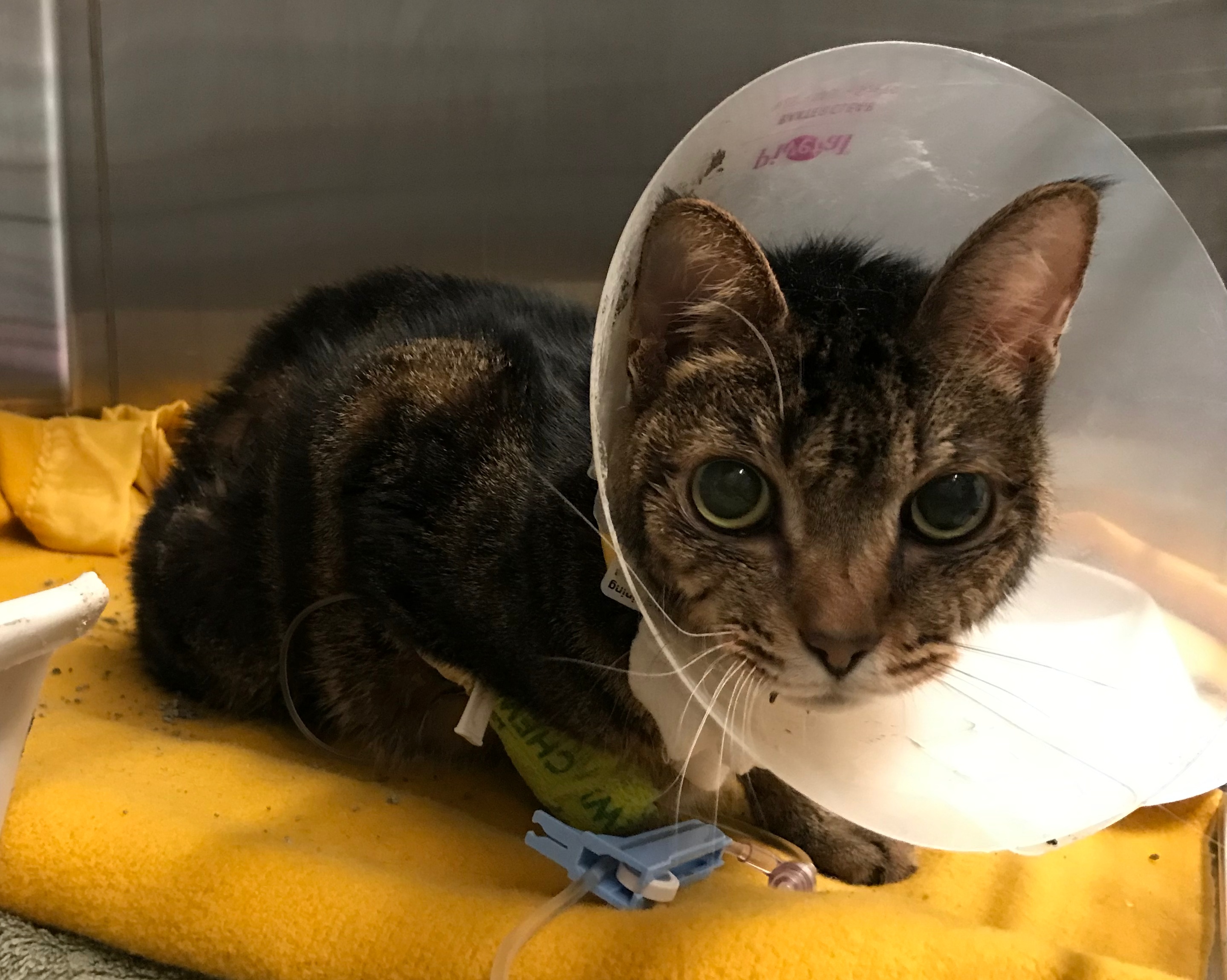
實在不知道為什麼,連續兩年柴犬都剛好在夏秋交替之際生了場大病。雖然最終都發現是因為亂吃東西造成的,並沒有長期的隱憂,不過仍然帶來了許多心力的折騰,也讓這篇文章的撰寫推遲了一陣子。
隨著Ph.D.進入最後一年,身邊許多好友接連畢業,剛入學的大學生和博士一年級學生,更是稚嫩的讓人感嘆時間的飛逝。和這些小朋友聊著他們對研究生活的憧憬,似乎看見了當年的自己,雖然心中有說不完的經驗想要分享,最終卻笑著決定還是讓他們各自慢慢探索吧!這樣說起來好像有點理解為什麼每次當我問Boaz建議時,他總是很簡單的說跟隨自己的熱情就好。
這一年發生了什麼?
這一年美國總算基本上恢復了原本的生活,從課程轉回實體、各種設施的開放到更多和人們實際的交流,彷彿回到了剛來美國的時候,一切充滿了希望和幹勁。不過雖然大部分事情看起來都往好的方向走去,我卻開始對研究方向感到了十分困惑。
在接觸了越來越多不一樣的領域(特別是量子物理和腦神經科學)之後,讓我開始思考什麼樣的方法論是我想要追尋的。不可否認的,數學還是對我來說最舒服自在的語言,每次看到一個新的數學猜想或是理論都還是常常讓我興奮得睡不著覺。但同時我也越來越能適應物理的直覺,以及生物的複雜世界觀。然而身為一個學者,在學習之餘,還是需要有所謂的研究產出,那麼我希望在哪個領域做出貢獻?我是要繼續做數學證明、跑數值分析還是做實驗提假說?
在學年剛開始時,我很確定的是,我暫時不太想繼續在還有很多小問題可以做的streaming model上面花時間,但是我又不太想要直接用很理論CS的方式做一些量子和腦神經科學的問題。於是,我開始系統性的讀一些物理的教材,同時在原本就有的腦神經科學讀書會更系統性的學習不同的方向。既然都進入了學習的模式,甚至乾脆做了Science and Cooking的助教,然後修了一直很想學的音樂理論。這些不同的學習除了在知識層面之外,很意外的還讓我接觸到了不同領域”做理論”的方式。由於是理論CS背景的關係,理論對於我來說一直都是“數學理論”,好像沒有了嚴格的數學證明就不太能登大雅之堂。但無論是在讀物理教科書時發現裡面幾乎不會有完整的證明、在Science and Cooking中看到了許多應用物理推導公式的神秘方法、還有音樂理論中許多約定俗成的瑣碎規則等等。我才漸漸理解並且接受“理論”可以有的多重面貌。
整個秋季下來學習了滿滿的知識,也讓我決定該找個機會好好整理一下所學。於是利用學校的資源在寒假的時候弄了一個為期兩週的迷你課程,趁機把未來的方向理清楚一些。在準備課程以及講授的過程中,我也漸漸對於跨領域研究有了不一樣的理解(在下面的段落會再深入討論),同時受到了Boaz不斷的提醒更是讓我意識到自己需要在許多的哲學性思考之餘,花更多的時間做實際的嘗試和工作(同樣的在下面的段落會再深入討論)。
到了春季學期,我更加深入的學習了量子計算和量子通訊,甚至還學了一些量子混沌及量子凝聚態。我突然意識到這些量子理論除了試圖解釋相對應的物理現象之外,更是提供了新的數學架構/語言能夠產生很多有趣的數學結構,這也是為什麼有些可以被應用在量子計算和量子機器學習上面。也許之後在其他的領域(例如腦神經科學),這些數學工具能夠刻畫一些實際現象。如果這樣的理論被建構出來了,並不見得是說大腦裡真的用了什麼量子物理,而只是說剛好某些大腦中的運作可以被同樣的數學描述和理解。
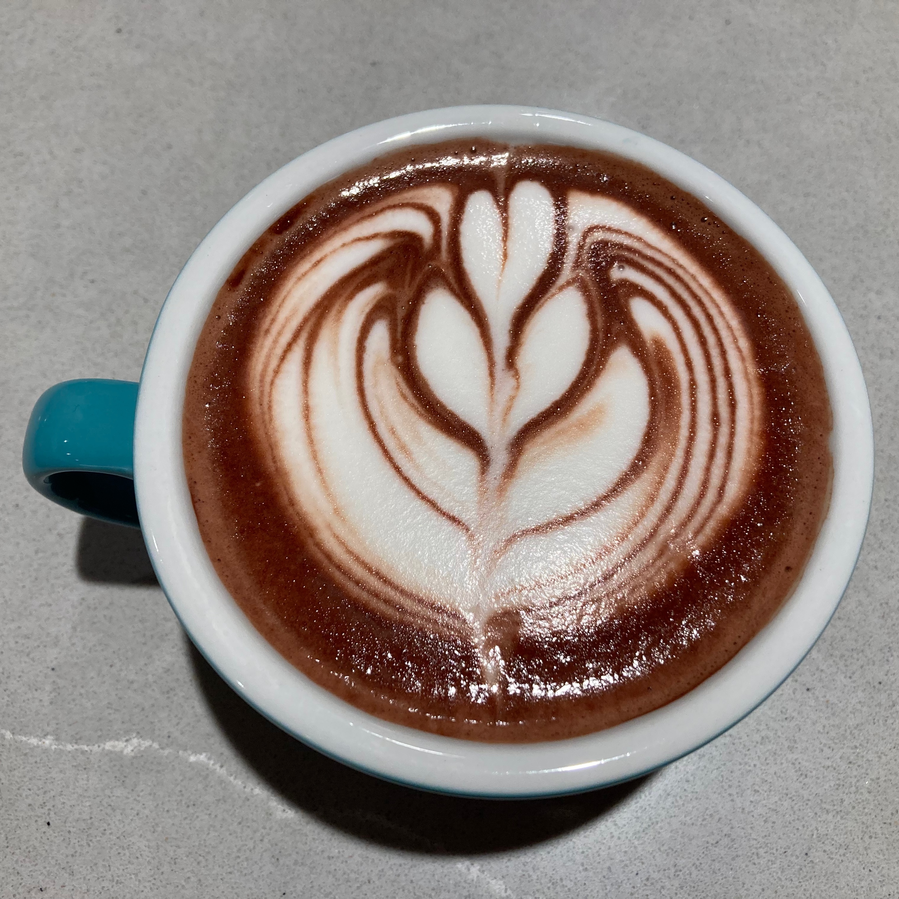
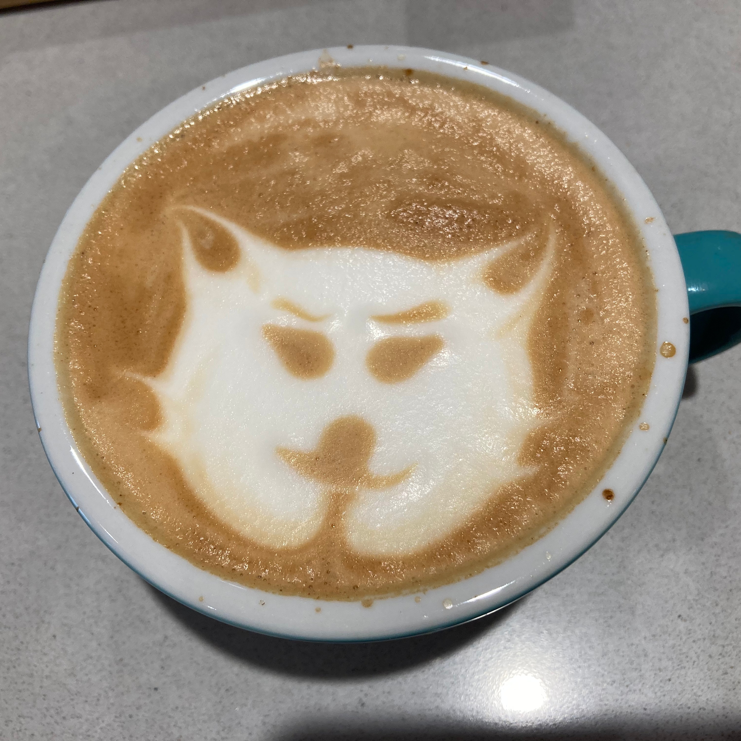
暑假我很幸運的到了紐約的Flatiron Institute的Center of Computational Neuroscience跟SueYeon做暑期實習。雖然大家都開玩笑説我學到最多的是怎麼做咖啡拉花,不過認真講,這十個禮拜讓我更全面的接觸了理論和計算腦神經科學的各種面向。最大的影響應該是讓我意識到了即使是要做腦神經科學相關的研究,我可能還是需要把由上而下的抽象理論,跟與實驗接觸的問題區分乾淨,才能夠各自找到合適的解讀和應用。
在博士即將畢業前這一年,很感謝Boaz給了我這麼大的自由探索不同的領域和方法論,雖然因為把大部分的時間都花在學習和思考上所以沒有太多研究產出,但是感覺漸漸找到了有熱忱和適合自己的研究方向。而平時的胡思亂想,也讓我把一些做(跨領域)研究和學生的癥結處整理出了一套自己的觀點。在剩餘的篇幅中,就讓我來分享一下近來的體悟。
從跨領域(interdisciplinary)到多領域(multidisciplinary)
一直以來,即使是在理論CS之內,我都是研究涉略範圍相對比較廣的人,也因此很自然地走上了所謂“跨領域”的道路。在開始跟越來越多其他領域(主要是物理和腦神經科學)的學者合作之後,我漸漸意識到,跨領域雖然能將一個領域的工具或方法應用在另外一個領域,但是卻時常有個隱形的阻礙。要嘛是不同領域的人之間的溝通一直不在同樣的頻率上,不然就是做出來的結果四不像。這樣的情形在比較明確的工具轉移(例如機器學習用在分析數據等等)時比較不容易出現,然而在比較抽象或本質的理論跨領域交流時(例如計算複雜度理論和量子物理)卻屢見不鮮。
這種阻礙通常都是來自於跨領域的合作太過於直接,會有其中一方把自己的方法論和專業整套搬去另外一個領域,沒有足夠的修改與溝通來適應對方的歷史脈絡跟價值觀。正因如此,讓我突然意識到更深入的跨領域合作其實應該要把“跨”這個字拿掉。畢竟有了“跨”這個動作時,說明了不同領域之間有主次之分,但是在真正深入的交流時,應該是要互相汲取適合的想法,融會貫通。也許,我們應該像牛頓那個時代之前的科學家看齊,事先進入不同的領域,學習其根本的概念與價值觀,甚至各自有些基本的研究經驗之後,在試著做多領域(multidisciplinary)的研究。
一個需要特別釐清的點是,我的意思並不是說大家應該先進入對方的領域花個幾年學成之後,在開始進行合作。我想強調的點是,在某些和多個領域有關的研究問題上,如果合作的成員們還沒有成熟到可以自如地在各個領域之間轉換時,那可能還不如選定其中一個領域,然後好好的以那個領域的方法論做下去。這甚至也適用在同一個領域的不同子領域的交流中!說來慚愧,會有這樣的體悟也是因為我自己和幾個不同的合作者,時常在不同的方法論之間(例如量子計算優勢(quantum computational advantage)的理論和實務層面)來回擺盪,幾個月下來常常搞得什麼進展也沒有。
當然,如果能夠有可以順暢溝通的合作者,也許就不需要自己真的從頭學起另外一個領域。不過身為一個理論學者,為了自己思想的自由,我還是期許自己可以腳踏實地的真的把物理和生物的基礎和價值觀內化吸收。這幾年下來,雖然離理想的狀態還有些距離,但是已經可以開始感受到自己的視野越來越廣闊,想問題的角度也越來越多,非常期待之後在不同領域打滾幾年甚至是做了博後之後,能夠在多個領域之間來去自如的境界。
性格的重要性
一個人到底適合做什麼?從小到大總是會有些人說是依照興趣,另外會有些人說是靠天賦。的確天賦是進入某個領域行業的入門券,隨著不同職業門檻可能會有所不同。興趣則可以說是讓一個人能夠在一個方向一直做下去的驅動力。而最近我開始越來越注意到另外一項因子的重要性,那就是性格。
性格有非常多的層面,例如在著名的MBTI性格測試中定義了四個性格的軸向(能量來源、感知偏好、判斷偏好、認知態度)。同時性格相較於天賦來說,更容易受後天的環境和經歷影響,雖然可能到了成年之後會越來越定型。
為什麼我越來越覺得性格在職業適合度上扮演關鍵性的角色呢?這也得從自身的經驗說起。在我的求學階段初期,我夢想的職業是打棒球,而最後棄武從文,一直以來的說法都是因為運動天賦不足。上了高中之後,一直對物理和數學很感興趣,但因為當時缺乏對這兩個學科真實面貌的理解,最後大學選擇主修了CS。在大學四年中我大量接觸各式各樣的領域,在CS內從軟體工程到Bitcoin到理論CS,在主修外也學了很多數學和旁聽一堆不同科系的課,還曾經弄了個跨領域讀書會,一度有超過十個不同科系的成員。大學畢業後,為了能夠繼續在學校學習知識,選擇了讀了個理論CS的博士班。五年過去了,從前兩年在理論CS內做了好多不一樣的子方向,到現在開始廣泛接觸物理和腦神經科學。
這筆流水帳看下來,我發現了一個共同的規律,那就是我的性格無法讓我只專注在一件小方向/事情上面很久很久。又或是說,當我掌握一項能力到一定程度之後,我就會開始被其他新的事物強烈吸引,進而轉換方向開始學習新的東西。即使隨著年齡的增長,我漸漸在做事情的細心和耐心上面成長了不少,但是我依然很難抗拒學習新事物的誘惑。這樣的個性讓我很難在需要極度專一的領域上走下去,而我也總是不知不覺的被拉往相對需要多種能力的方向。
當然,性格不是只有一個面向,其他諸如好奇心、追根究底的精神、好勝心等等也都是帶著我一直走到現在不可或缺的角色。看看身邊的研究生同學和朋友,也許外人會覺得大家的共通點是所謂的“聰明”,但我反而覺得對熱愛事物的堅持才是這些博士生還有學術工作者的必要條件。
哲學思考與實際工作的平衡
年初有次在和Boaz聊天討論研究方向的時候,Boaz突然脫口而出,要我小心不要變得太像一個哲學家。我當時一直沒有很理解他的話,在我心中,一個好的科學家不是也應該需要花一定程度的時間做哲學思考,釐清楚自己工作的意義和貢獻是什麼嗎?
直到最近在翻Steven Weinberg寫的To Explain the World: The Discovery of Modern Science,才讓我重新思考了關於哲學和科學的差別。Weinberg從古希臘哲學家例如柏拉圖和亞里斯多德講起,提到在那個年代其實就已經有非常多關於對世界如何運作的“理論”,思想和學問的累積也是很有深度,那為什麼這些知識是被歸類為哲學?或是為什麼這些哲學無法帶給古希臘科學革命?我們又可以如何從他們身上學習到借鏡?
也許直接拿哲學和科學相比,實在會有太多的不同,不過我覺得真的要說的話,兩者之間有兩個根本的差異:首先是科學講求驗證,再來就是科學(在理想上)追求盡可能的客觀和共識。對於後者可能會牽扯一些不同科學哲學流派的不同解讀,所以在這邊我想要只討論第一點,驗證在科學中扮演的重要角色。
說到驗證,其實仍然避不開哲學的討論,尤其是像對於複雜系統或是高能物理等等,這些科學的子領域的確可能無法再看得見的未來有可能被嚴謹驗證。然而這邊我想強調的更是科學中一種“驗證的態度”。即使是研究複雜的腦神經科學,或是宇宙起源及大統一理論等等,即使大家都知道短期內不太可能有實驗能夠驗證檯面上的理論,但是多數主流的發展仍然會抱持著盡可能接近實驗的精神和態度。從學術界的兩大期刊,Nature和Science,基本上都要求要有實驗的潛規則中,就可以看出驗證在科學界中的核心角色。
而這種對驗證態度的要求,讓科學相較於哲學是非常的實務的,也就是大家會傾向於看到證據和實際的“工作結果”。這樣的工作結果可以是進行嚴謹的實驗,也可能是詳細的數學理論推導。縱使方法論因為研究的課題不同,會略有差距,但共通點就是強調“做”。譬如說前幾週和一個做量子重力理論的博士後聊天,他就跟我說,就算你有再多天馬行空的理論和想法,最終還是要回到計算來讓人信服。雖然這些數學理論還沒辦法在物理世界中被驗證,但是至少要能夠在數學世界中說服人!
回到Boaz給我的提醒,的確哲學思考固然可以提升思想的深度,但是也很容易落為眼高手低。人生有限,我選擇的又是一條科學/數學的道路,應該是要以工作和創造為主,天馬行空和自我批判為輔。就像許多人說的,最理想的學者狀態,也許就是個白天的科學家和晚上的哲學家吧!?
27 May 2022
趁著六月要去實習前的空擋,跑來參加了Simons Institute十週年研討會。研討會包含了二十個左右橫跨各種主題的演講,以及幾個討論理論CS未來發展的座談會。由於年底就要開始想想下一步要往哪裡去了,這個研討會可以說是一個讓我想清楚下個階段研究方向的的好機會。
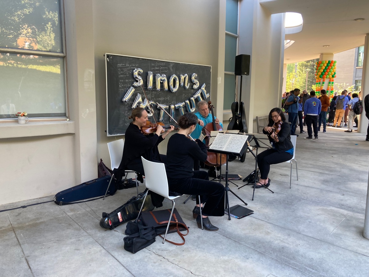
首先不得不說這次Simons十週年研討會讓我對理論CS有了全新的認知,原本抱持著參加類似STOC/FOCS這種會議的心態,預期大部分的演講應該都是著重複雜數學技術。沒想到我完全跌破了眼鏡,整整三天下來(我第一次在一個會議中聽了所有的演講),不光是主題的多樣性,連研究方式的豐富程度也讓我大開眼界。尤其是大部分的講者除了呈現了他們想要解決的研究問題和成果,更是在不自覺中展現了他們面對各自遇到的困難問題時,不同解決問題的方法論。在前往Berkeley的路上時,我還在想該如何問問大家對於數學證明之外的理論研究的方法論有沒有什麼看法,在聽了這些演講後,這個問題還沒被問出就被回答了。
而這幾年來我心中對理論CS發展方式的批判和質疑,也在會議劃下句點時跟著煙消雲散。我才終於發現到雖然會議中的主流文章越來越加複雜和脫離實際,但是還是有著一群領域內的大佬們試圖發展不同的方式,用理論的角度來試圖回答一些數學證明不太能觸及的問題。這邊我要澄清一下我還是非常喜歡數學證明,平常更是會不時學一些新的數學理論(像是上週末看了好多的代數拓墣),不過同時我覺得數學證明不見得在所有跟計算相關的問題上都能夠得到令人滿意的解釋,甚至有時候過度追求完美的數學證明反而會失去了深刻的見解。
在聽了第二天下午的panel discussion以及和幾個前輩聊聊之後,更是讓我對於未來中長期的研究方向/方法論有了更成熟的圖像,感覺就像是重新地愛上了理論CS這個領域,對於未來充滿了興奮與期待。
對於「理論」的重新思考
語言真的是個很奇妙的東西,當年紀越來越大,很多詞彙的定義對我來說反而變得越來越模糊不清了。而「理論」大概就是一個很好的例子吧!(另一個讓我最近花很多時間思考的是「科學」)
年輕的時候,「理論」之於我來說就是抽象的邏輯推導建模,也就是設立基礎公設/公理/定義,然後從一系列的邏輯推演中得出理論理解。而理論CS的基礎教育也全部都是使用provable analysis,只有數學定理才能被稱之為理論。然而,這就是做理論唯一的方法嗎?或是讓我們退後一步,到底什麼是理論?理論的目的/意義/影響是什麼?理論可以有什麼樣的形式?
理論是什麼?
我很喜歡Wikipedia上對理論(Theory)的定義:
A theory is a rational type of abstract thinking about a phenomenon, or the results of such thinking.
理論是關於一個現象的理性抽象思考,或是其產物。
但也許這個定義有點太哲學了,讓我們試著以它做為起點,來拼湊看看一些關於「理論」更具體的描述和性質。我認為,一個理論是個對於某些現象或是概念的知識體系。而這個體系中主要包含了(1)一套理論語言(2)知識形成和驗證的機制。
理論語言:說到一個理論使用的語言,可能馬上想到的就是相關學科的一些專有名詞。的確這是語言最基礎的一個層次,但理論語言通常可以提供遠遠高於定義層次的作用。
首先理論語言提供了一個思考事情的方式。例如達爾文的天擇論,提供了一套十分生動的語言,用擬人化(競爭/適者生存)的方式讓生物學家(甚至一般人)來思考和討論物種的演化。另外一個我很喜歡,但是可能比較需要一些數學經驗的人才能體會的例子是範疇論(category theory)。長話短說,範疇論提供了一套非常乾淨簡潔的語言,讓數學家可以用同樣的方式理解許多原本看似距離遙遠的數學概念。
更進一步,理論語言提供了一個領域規劃未來研究方向的基石。以電腦科學為例,計算複雜度理論(computational complexity)提供了複雜度類別(complexity classes)這套語言,讓人們可以非常具體的指出領域內重要的問題是什麼(e.g., P versus NP)。反觀一些還很缺乏理論語言的領域,諸如「什麼是intelligence?」等問題,會讓研究學者非常難以嘗試回答,因為甚至沒有什麼著力點。
而一旦理論語言被確立了之後,其實同時也為一個領域能夠回答的問題設了一個上限。就像哥德爾不完備定理(Gödel’s incompleteness theorems)告訴我們的,一個完善的邏輯系統總是有他無法解釋/證明的命題。即使是對非形式化的語言,我相信同樣的極限也是存在的,只是可能更難清晰的論證出到底那個極限在哪裡。
知識形成和驗證的機制:一個理論體系除了語言之外最重要的大概就是一套驗證知識的機制了吧!換句話說,就是該如何系統性且客觀理性地判斷什麼樣的論述可以被留存下來。
隨著所探討的學科和理論語言的不同,甚至和歷史發展或是學者的風格,每個領域的驗證機制或多或少都有些異同之處。而我認為大部分的驗證機制都可以被歸類為以下兩種類型的其中一種,或是在兩者中取了某種平衡:
形式方法(formal method):
首先其實我原本想用的詞是「分析方法(analytical method)」,但是考量到一些領域對於分析方法有不一樣的詮釋,我決定用個比較不容易產生誤會的詞來解釋我想表達的概念。
對我來說,形式方法的論證機制的特徵是著重在根據一些共同認定或是假設(axioms/hypotheses)的基礎之下,使用數學證明和邏輯推演論證出更多的定理(theorems),並且在眾多定理之下繼續往前推導出更多新的定理。而這些定理,以及人們對定理的詮釋,則構成了知識。在許多時候,推導定理的過程會產生一些意想不到的驚喜,而使得這些過程/數學證明往往也會成為知識的一部份。
數學毫無疑問地就是使用形式方法的最佳例子,而理論CS中大部分的子領域也都是使用這樣的方法論。在一些自然科學的理論分枝,像是一部份的理論物理或是理論生物研究,也會或多或少採用形式方法。
形式方法的優點在於,除了邏輯的嚴格性之外,它沒有太多其他的限制,因此有時候可以帶領人們思考地非常遙遠。很多的例子可以在理論物理中見到(e.g.,相對論、量子力學),而在理論CS之中,許多有趣的概念也是受益於這樣自由的思考模式(zero-knowledge proof, probabilistic checkable proof)。不過這個優點的反面就是很容易受到完美邏輯論證的限制綁手綁腳,或是為了數學上的正確必須用非常冗長瑣碎的證明解釋一些其實很簡單的概念。
經驗方法(empirical method):
絕大多數的科學學科(包括其比較理論的分枝)採用的都是經驗方法,也就是透過實驗觀察,或是數值模擬的方式來搜集事實(facts)及驗證假說。當然根據不同的學科和問題,會有不同的子機制(e.g.,不同的統計方法)來檢視什麼樣的觀察是合理的,在這邊我想強調的比較是經驗方法的最底層次是現實經驗,這也是為什麼我把數值方法歸類於此而非獨立成第三類驗證機制。
經驗方法與形式方法最大不同的地方就在於,它提供了事實(facts),它告訴了我們且試圖解釋真實發生的實情。雖然經驗方法得出的一切觀察與理論都還是參雜了一些人為的推論的解讀,但是本質上它是服膺於實際發生現象。也因此,經驗方法的底線是(在論證”合理”之下)符合和解釋現實。
So what?
寫了這麼多看起來像是廢話的東西,我們終於可以來討論我對「理論」重新思考的重點了。由於我其實也還在塑建自己想法的過程中,所以以下我將會用提出問題的方式來呈現我的思考,希望可以激發讀者做一些深入的思考,也期待這些問題可以漸漸地找到一些有意思的回答。
現有理論方法論的邊界?私認為現有的理論方法論走到了兩個轉捩點。其一是形式方法進入到了近乎巴洛克風格的階段,越來越複雜且和現實脫離。其二是機器學習/深度學習帶來經驗方法的革命,各種人類無法理解但是實際上有效的方法(e.g., Alphafold)大量湧現。前者警示了我們傳統完美數學邏輯論證的方式似乎進入了緩慢成長且窄門化的境界,後者則是挑戰了現有理論方法能夠處理的邊界。我們是否真的能依賴一直以來的方法論們來處理這些舊時代遺留的重要問題和新時代產生的新問題?我們是否需要新的理論架構?
如何構造不同層次的理論語言?對於上述的問題,我個人認為的突破口是建立一系列服務不同層次理解的理論語言。現有的理論語言大多要麼是純粹數學邏輯化的,要麼是描述性(descriptive)的,鮮少能有介於之間且能夠順暢翻譯的語言。一個好的例子可能又是達爾文的天擇論,這個理論架構中不但有一套比較方便溝通類比的直覺性語言(e.g., 適者生存),同時有比較機械化的中層語言(e.g., 適應性地貌(fitness landscape)),還有底層的數學語言(e.g., 演化動力學(evolutionary dynamics)){:target=”_blank”})。對於那些卡在底層數學證明的問題,我們是否能夠往上一層建立個不完美但堪用的理論語言?
有什麼混用形式方法與經驗方法或是其他的方法論?物理學可以說是最成功將純粹抽象數學推導和實驗觀察結合的學科,其他的領域是否能夠也有這樣混合並用的方法論?其實每個領域或多或少都有不同程度的混用這兩種截然不同的方法論,只不過子領域之間的隔閡造成不良的溝通。而根本的原因可能還是目的與審美的不同,導致形式方法與經驗方法漸行漸遠。也許要形成新的方法論沒有想像中那麼的難,真正的挑戰反而是在於如何接壤過去舊有的學派,展開心胸接納不同的方法。
22 Jan 2022
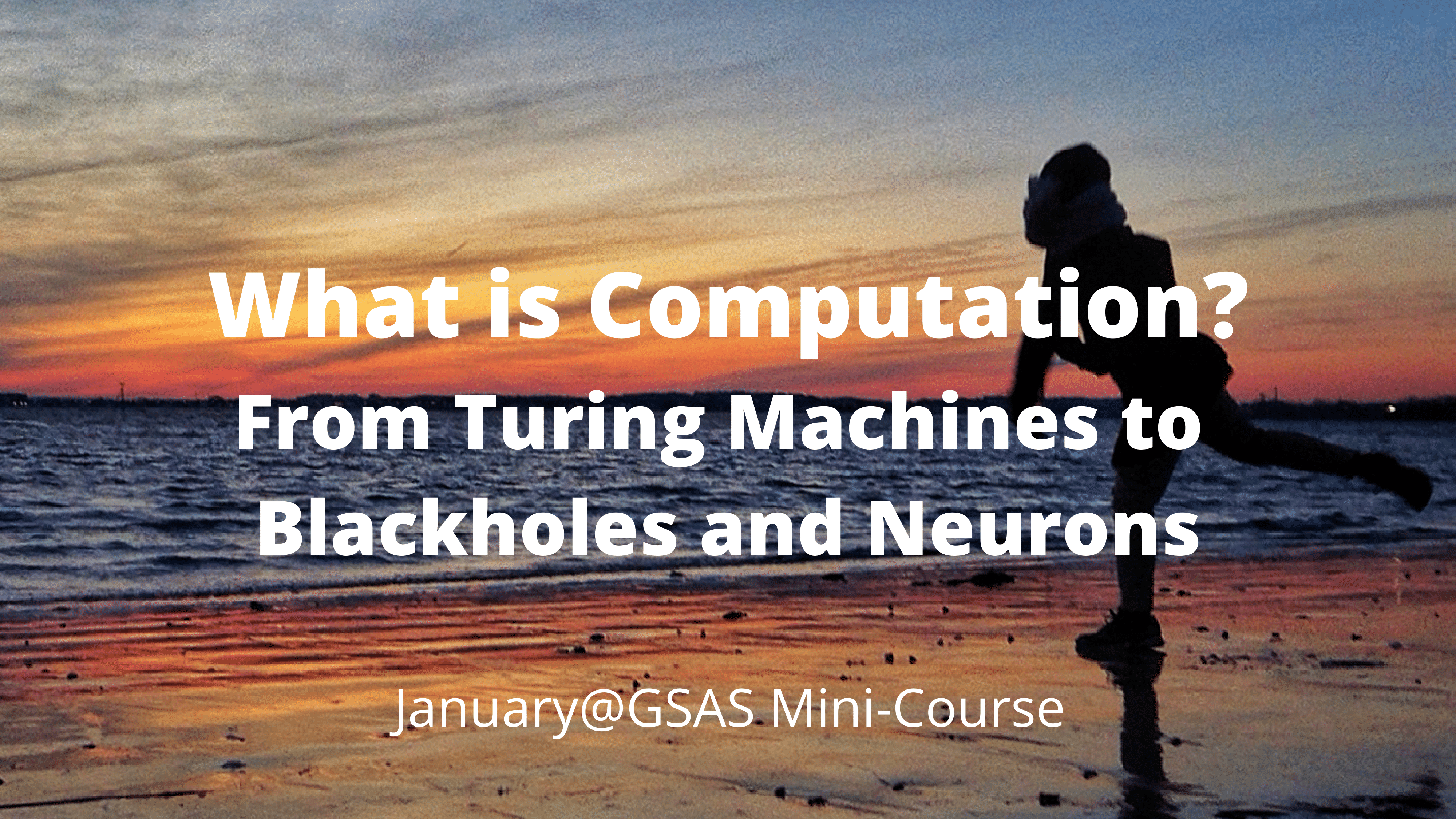
(See here for an English version)
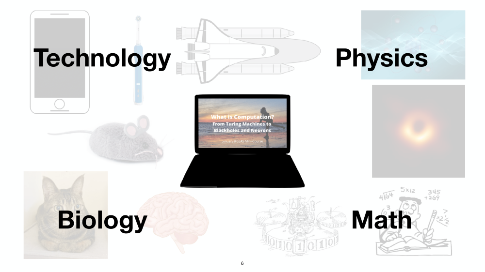
這一個月來幾乎八成的時間都是在準備這個為期兩週的mini-course,未料在最後幾天,一個小插曲讓我重新認真思考了一下科普的本質倒底為何?我們真的需要科普嗎?科普會不會反而讓科學的進展開倒車?
先讓我們試圖釐清科普的定義吧!仔細想想的話,科普可是有非常多不同的形式和層級呢!
新聞媒體:“達爾文進化論被推翻了!”,這大概是一般人生活中最常接觸到的科普吧?各種新聞媒體到網路影片工作者,每天都有無數的人試著把最前沿的科學研究用淺顯易懂的方式傳達給大眾。當然這種形式的科普品質十分參差不齊,在市場競爭的叢林中,有些人靠聳動標題維生,有些人則是堅持專業獲得死忠粉絲。
科普書籍:如果更有一些時間和心力,一般人接下來會接觸到的大概就是科普書籍了。同樣的,書店中科學區的書架上,琳琅滿目,各種名人以及得獎科學家的加持,範圍更是從物理、化學、數學到生物、心理學等等。跟新聞媒體最大不同的地方是,科普書籍通常具有較完整的系統,有些甚至一出手就是四、五本一套。然而畢竟不是教科書,面向的是普羅大眾,科普書籍通常還是使用非常淺顯的敘述,不會假設太多的教育背景,很多時候甚至會省略掉一些有點重要的概念。
線上課程:有時候還真的挺羨慕現在的小朋友,在網路上很輕易的就可以免費看各種大學教授開設的線上課程。儘管許多時候這些線上課程被簡化了許多,但是透過作業以及網路論壇互動,甚至是簡單的實驗,是可以獲得科普書籍無法做到的學習效果。
大學通識課程:這也許是科普中最高的層次了吧?在大學通識課程中,教授們不但有整個學期的時間,同時學生們受過基本教育的訓練,即使可能來自稍微不同的背景,但是相對於一般民眾,可以假設這些大學生具有流暢的邏輯思辨和溝通能力。例如我在上學期助教了一門「Science and Cooking」的通識課(這門課同時也有線上版本,但是簡化了非常多),老師們在短短三個月中,讓來自不同學院的學生們淺嚐了諸如elastic modulus、diffusion equation等等在(初階的)專業課程中才會學到的基本概念。
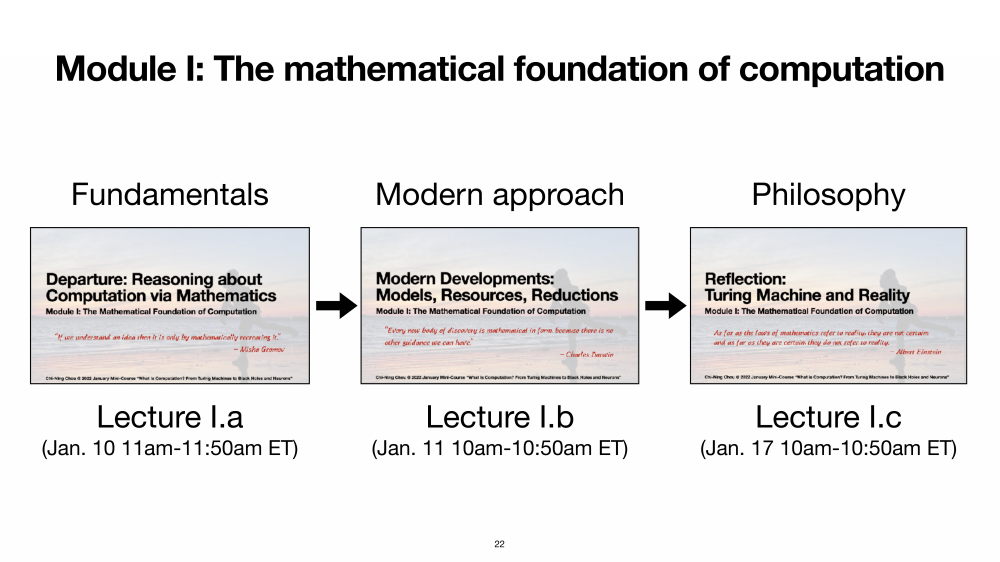
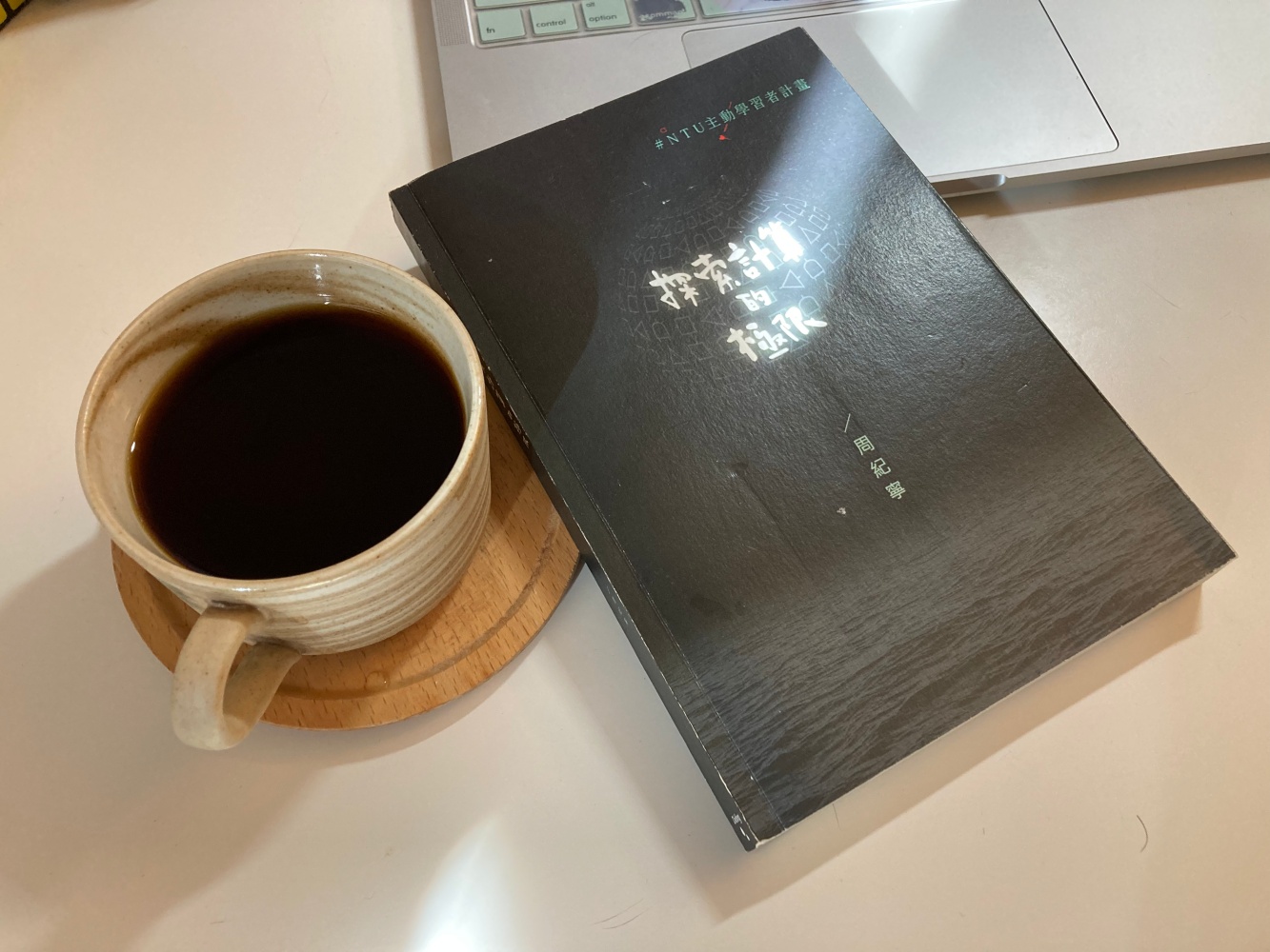
至於我的mini-course在哪個層級呢?我自認為大概是介於線上課程和大學通識課程之間,因為課程內容在廣度的要求之下相對犧牲了深度,但是同時我也期許自己能夠盡可能的放入很多精髓讓學生在未來可以繼續探索。而下一步我也打算著手寫一本相關的科普書籍,希望用不同的形式呈現我對這些跨領域知識的理解和看法。
科普的目的是什麼?
我想每個人可能都對科普的目的有略微不同的看法,有些人覺得是為了讓艱澀的科學知識更容易讓大眾接觸,有些人覺得這是個很好增加知名度的方式,有些人可能是很享受教學和寫作的過程。
不過以我的例子來講,其實說來慚愧有點自私,最初的原因主要有兩個:首先是這樣可以讓我身邊的家人和朋友更知道我在做什麼,像是我在大學畢業前寫了一本「探索計算的極限」,講解了基本的計算理論概念,最後分送給朋友和家人。雖然最後我爸媽好像還是沒有看完,不過至少例如我的設計師好友小羊,在完全沒有相關背景的情況下,花了半年的時間讀完後,現在大約知道二進位制和圖靈機是什麼了!第二個原因則是透過科普的寫作,其實對我自己來說是一個沉澱和昇華的過程。在之中我會不斷地挑戰自己最底層的理解,接著試圖猜測潛在讀者可能會困惑的地方,在一來一回中琢磨出連我一開始可能都意想不到的敘事和理解方式。
但是這樣的動機的確可能還是稍嫌薄弱,看看我在這個mini-course所花費的心力,似乎不成比例。的確,另外一個科普(還有教育in general)帶來很大的附帶品就是和聽眾/讀者/學生的互動。這種互動和前述有些人追求的知名度是不一樣的,更像是一種找到知音的快樂。話說回來,終究還是自私的讓自己開心。
難道對我來說科普的目的就只有這樣嗎?如果站在客觀一點的角度來看,我是有些話想說。
首先我認為在現在的教育體制下,知識還是非常分配不均的。我一直到進了台大之後,才發現高中以前我竟然錯過了這麼多,如果當你連碰到好的書和教材的機會都沒有,那麼再怎麼聰明的人也是無法從無到有變出人類累積千百年的智慧。而到了Harvard之後,我更驚覺big picture的重要。當先建立了好的基礎觀念以及了解一個領域的大方向結構和價值觀,學東西的效率完全是提升好幾個層級。然而無論是好的教材或是big picture,即使在現在網路發達的世代,仍然還是沒有那麼容易讓一般人接觸到。
Everything should be made as simple as possible, but not simpler.
所有事物都應該被盡可能的簡化,但是不能簡化過頭。
- Albert Einstein.
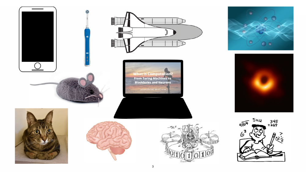
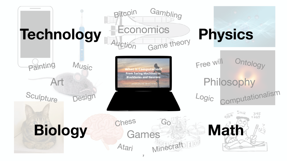
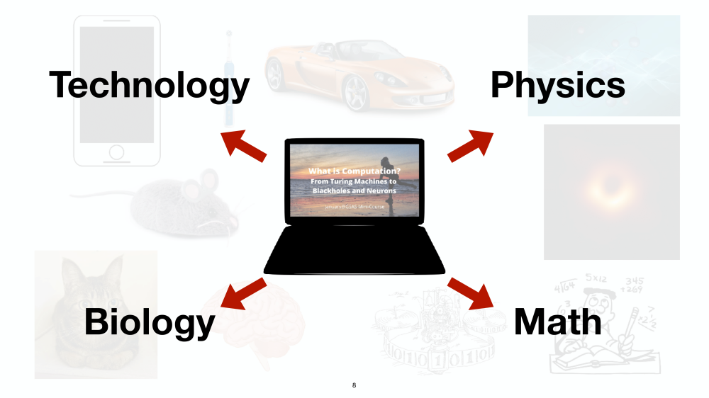
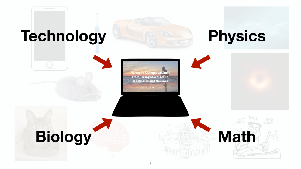
此外,我覺得科普在現代社會還有另一個特殊的角色,那就是增進領域之間的交流和學習,這也是我這門mini-course的核心價值。在當今各個領域都蓬勃發展,且變得越來越複雜艱澀之後,跨領域學習面對的牆變得越來越高越來越厚。同時跨領域互動的目的也和本科學習的目的有些不同,更多的是在交流彼此的核心概念,藉此激發出在各自領域的新想法。
科普的危險
接下來讓我們進入本文的核心討論:科普是不是危險的?
以我的觀察來看,認為科普產生弊大於利的論證,主要著重在於(1)科普會讓一般人有種覺得懂了很多的錯覺(2)科普讓人變得懶惰而不扎實的學習(3)科普過度簡化甚至可能造成科學進展的倒退。
首先我非常認同前兩點,一些“不好”的科普的確很容易衍生這樣的社會問題。但是我也想指出這種論證的一個盲點:會因為讀了科普而產生懂很多的錯覺或是對學習懶惰的人,他們並不會因為沒有了科普就變成一個上進的人!相反的是,如果有個好的科普,能夠讓人在學習的過程中反而更發現自己的無知,這樣反而達到正面效果,人們會因此更知道自己缺乏什麼而繼續學習。而這也完全是我在我的mini-course想要跟學生們傳達的!在這邊也跟大家分享一個我不斷跟學生強調的一個quote:
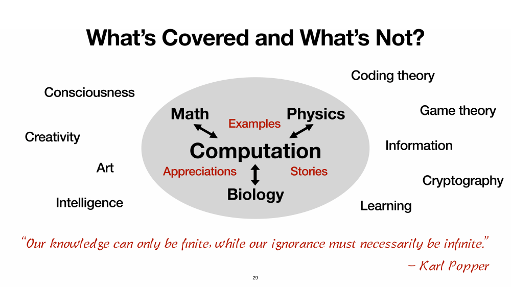
Our knowledge can only be finite, while our ignorance must necessarily be infinite.
我們的知識只能是有限,同時我們的無知必定是無限。
- Karl Popper.
所以對我來說,(1)和(2)更像是對科普推廣者的提醒,而非真正的危險。
至於(3),這個就非常的subtle了,身為非常資淺的學術工作者,我在這邊只敢提供一些小小的評論,同時希望可以激起更多對於類似議題的討論!
首先,科學是不斷地進步的嗎!?沒辦法讓科學”進步”的就不配被稱為好的知識或研究嗎?如果是一直身在學院的象牙塔中,一路吸收所謂“正確”的科學知識,那麼的確看似只要跟最後留下來的理論不相符的都可以被稱為沒用。然而這絕對不是科學發展真實的面貌,綜觀科學史,現在最終留下的理論,很多是奠基在如今被視為不那麼正確,或甚至在當初有些誤導人的理論。而在科學發展的前沿,我們也知道許多如今被視為傑出的理論,在一開始通常也都是在許多略有錯誤的理解和猜想中,慢慢修正孕育出來的。
最後,我個人認為,把科學的論述單一化是非常危險的,這樣反而更容易阻礙科學的進展!讓我們從演化的角度來看看,如果沒有什麼變異,那麼雖然現在這個理論把世界解釋的很好,但同時也意味著改變或”往前”的動力是比較小的。反觀在變異大的情況下,縱使會先產生許多被淘汰掉的變種,甚至走倒車,但是需要透過這些變異,才可能讓我們更有機會產生下一個“典範轉移”!
自我省思與期許
寫到這邊,我希望我至少能夠暫時說服讀者如果有“好的科普”,那麼對於社會、科學發展、跨領域交流,都是利大於弊的。不過最終就必須正視我所謂“好的科普”是什麼?會不會這樣的理想在現實中是不可行的?該如何分辨科普的優劣?
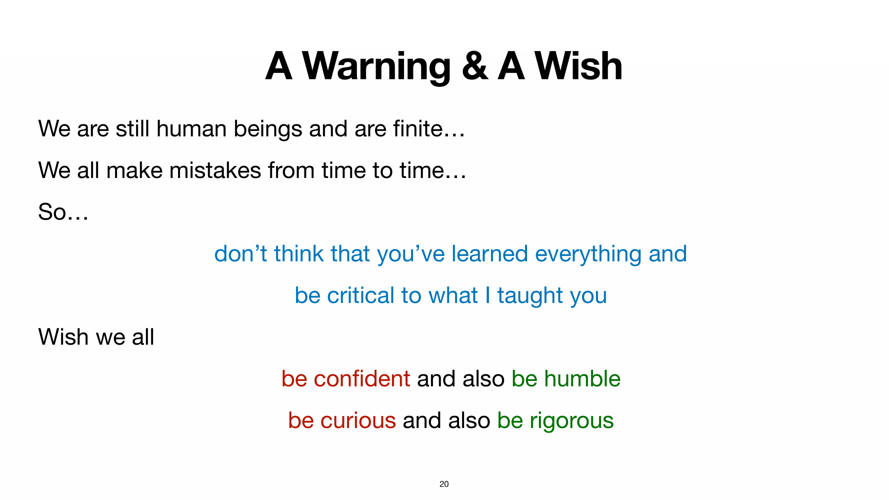
我覺得,一個“好科普”的必要條件,是清楚地讓讀者或學生知道有什麼東西是被省略的、有什麼東西是我們還不知道的。畢竟知識本身最終還是由接受的一方詮釋,再好的老師或是再好的書,都無法控制別人如何解讀(同時這也是科學非常“社會化”的一面)。於是在知識本身的呈現之外,適時的提醒便顯得非常重要。其實話說到底,即使離開科普的討論,在科學的學習和研究中,抱持謙卑和清楚地知道自己不懂什麼,也是不可或缺的。下圖是個我的mini-course中最後一堂課中的投影片,在這邊作為一個警惕與期許。
至於理想中的好科普是否在現實中可行?我覺得這個問題就像是在問科學家是否可以找到理想中的完美理論一樣,到頭來可能更接近於個人信仰了。至少我個人是保持樂觀,在市面上的確也看到一些對我來說還不錯的書或是課程。但至於該如何辨別科普的優劣,這個可能真的就只能靠個人修煉了。任何的書或是課程,都是會有正面和負面的聲音同時出現,有時候正面音量大也不見得代表就是好的,反之負面音量大也不代表一無可取。最終雪亮的眼睛以及批判的閱讀,才是能夠帶領一個人在知識之路顛簸向前的路燈。
最後,也想留幾句話給未來的自己作為一個警惕。在受到刺激的時候,別急著反駁,甚至不小心忘記了檢視自己的問題。人都會犯錯,最重要的是坦然面對自己的錯誤,並且在之中成長。期許自己,be confident but also be humble, be curious but also be rigorous。