Research
I am a scientist and theorist working in computer science, physics and neuroscience. My main research interest is to understand the fundamental limits of computation (and/or beyond, e.g., intelligence) in different (complex) systems including artificial/mathematical, biological, and physical.
My academic journey began in theoretical computer science, specifically in computational complexity theory. This field adopts a bottom-up approach, striving for provable asymptotic understandings within computational models like Turing machines and circuits. In recent years, my interests have expanded to encompass (statistical) physics and neuroscience. These disciplines lean more towards a top-down approach, constructing observables and phenomenological models to elucidate nature and the workings of the brain. I value both these approaches for tackling challenging scientific questions and firmly believe in the symbiotic relationship between theory and practice.
At present, my primary research area is neuroscience. For a deeper dive into my work, please refer to the subsequent introductions detailing each of my research directions.
Neural Representational Geometry
Neuroscience Active
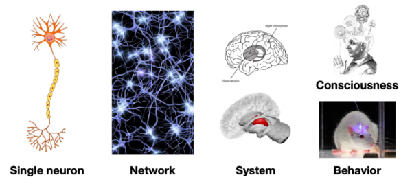
Neurons in the brain generate patterns of activity in response to external stimuli or while an animal is performing a task. These patterns, known as neural representations, are pivotal for understanding how the brain encodes information and performs computations. As we transition into an era of large-scale neural recordings, the need to decipher complex, high-dimensional, and noisy neural representations demands the development of new modeling and analysis frameworks to facilitate quantitative investigations.
The central theme of this research direction will be the development of quantitative foundations for neural representations, which emerge from learning and dynamics in neural circuits. We will utilize principles and methods from geometry, computation, and physics, and apply them to design testable hypotheses for experiments aimed at investigating the brain’s mechanisms at the population level.
[Related papers ]Diagnosing Generalization Failures from Representational Geometry Markers
Chi-Ning Chou, Artem Kirsanov, Yao-Yuan Yang, SueYeon Chung.
International Conference on Learning Representations (ICLR 2026).
[arxiv] [conference version] [abstract ] [bibtex ]
@inproceedings{
chou2026diagnosing,
title={Diagnosing Generalization Failures from Representational Geometry Markers},
author={Chi-Ning Chou and Artem Kirsanov and Yao-Yuan Yang and SueYeon Chung},
booktitle={The Fourteenth International Conference on Learning Representations},
year={2026},
}
Generalization—the ability to perform well beyond the training context—is a hallmark of biological and artificial intelligence, yet anticipating unseen failures remains a central challenge. Conventional approaches often take a "bottom-up" mechanistic route by reverse-engineering interpretable features or circuits to build explanatory models. While insightful, these methods often struggle to provide the high-level, predictive signals for anticipating failure in real-world deployment. Here, we propose using a "top-down" approach to studying generalization failures inspired by medical biomarkers: identifying system-level measurements that serve as robust indicators of a model’s future performance. Rather than mapping out detailed internal mechanisms, we systematically design and test network markers to probe structure–function links, identify prognostic indicators, and validate predictions in real-world settings. In image classification, we find that task-relevant geometric properties of in-distribution (ID) object manifolds consistently forecast poor out-of-distribution (OOD) generalization. In particular, reductions in two geometric measures—effective manifold dimensionality and utility—predict weaker OOD performance across diverse architectures, optimizers, and datasets. We apply this finding to transfer learning with ImageNet-pretrained models. We consistently find that the same geometric patterns predict OOD transfer performance more reliably than ID accuracy. This work demonstrates that representational geometry can expose hidden vulnerabilities, offering more robust guidance for model selection and AI interpretability.
Feature Learning beyond the Lazy-Rich Dichotomy: Insights from Representational Geometry
Chi-Ning Chou*, Hang Le*, Yichen Wang, SueYeon Chung.
International Conference on Machine Learning (ICML 2025).
Selected for Spotlight Presentation.
[arxiv] [conference version] [abstract ] [bibtex ]
@inproceedings{CLWC25,
  title={Feature Learning beyond the Lazy-Rich Dichotomy: Insights from Representational Geometry},
  author={Chi-Ning Chou and Hang Le and Yichen Wang and SueYeon Chung},
  booktitle={Forty-second International Conference on Machine Learning},
  year={2025}
}
Integrating task-relevant information into neural representations is a fundamental ability of both biological and artificial intelligence systems. Recent theories have categorized learning into two regimes: the rich regime, where neural networks actively learn task-relevant features, and the lazy regime, where networks behave like random feature models. Yet this simple lazy–rich dichotomy overlooks a diverse underlying taxonomy of feature learning, shaped by differences in learning algorithms, network architectures, and data properties. To address this gap, we introduce an analysis framework to study feature learning via the geometry of neural representations. Rather than inspecting individual learned features, we characterize how task-relevant representational manifolds evolve throughout the learning process. We show, in both theoretical and empirical settings, that as networks learn features, task-relevant manifolds untangle, with changes in manifold geometry revealing distinct learning stages and strategies beyond the lazy–rich dichotomy. This framework provides novel insights into feature learning across neuroscience and machine learning, shedding light on structural inductive biases in neural circuits and the mechanisms underlying out-of-distribution generalization.
The Geometry of Prompting: Unveiling Distinct Mechanisms of Task Adaptation in Language Models
Artem Kirsanov, Chi-Ning Chou, Kyunghyun Cho, SueYeon Chung.
Annual Conference of the Nations of the Americas Chapter of the ACL (NAACL 2025).
[arxiv] [conference version] [abstract ] [bibtex ]
@inproceedings{KCCC25,
title={The Geometry of Prompting: Unveiling Distinct Mechanisms of Task Adaptation in Language Models},
author={Artem Kirsanov and Chi-Ning Chou and  Kyunghyun Cho and SueYeon Chung},
booktitle={The 2025 Annual Conference of the Nations of the Americas Chapter of the ACL (NAACL 2025)},
year={2025},
}
Decoder-only language models have the ability to dynamically switch between various computational tasks based on input prompts. Despite many successful applications of prompting, there is very limited understanding of the internal mechanism behind such flexibility. In this work, we investigate how different prompting methods affect the geometry of representations in these models. Employing a framework grounded in statistical physics, we reveal that various prompting techniques, while achieving similar performance, operate through distinct representational mechanisms for task adaptation. Our analysis highlights the critical role of input distribution samples and label semantics in few-shot in-context learning. We also demonstrate evidence of synergistic and interfering interactions between different tasks on the representational level. Our work contributes to the theoretical understanding of large language models and lays the groundwork for developing more effective, representation-aware prompting strategies.
Geometry Linked to Untangling Efficiency Reveals Structure and Computation in Neural Populations
Chi-Ning Chou, Royoung Kim, Luke Arend, Yao-Yuan Yang, Brett Mensh, Won Mok Shim, Matthew Perich, SueYeon Chung.
Under review.
[bioRxiv] [abstract ] [bibtex ]
@article {Chou2024.02.26.582157,
  author = {Chou, Chi-Ning and Kim, Royoung and Arend, Luke and Yang, Yao-Yuan and Mensh, Brett D and Shim, Won Mok and Perich, Matthew G and Chung, SueYeon},
	title = {Geometry Linked to Untangling Efficiency Reveals Structure and Computation in Neural Populations},
  elocation-id = {2024.02.26.582157},
  year = {2024},
  doi = {10.1101/2024.02.26.582157},
  publisher = {Cold Spring Harbor Laboratory},
  journal = {bioRxiv}
}
From an eagle spotting a fish in shimmering water to a scientist extracting patterns from noisy data, many cognitive tasks require untangling overlapping signals. Neural circuits achieve this by transforming complex sensory inputs into distinct, separable representations that guide behavior. Data-visualization techniques convey the geometry of these transformations, and decoding approaches quantify performance efficiency. However, we lack a framework for linking these two key aspects. Here we address this gap by introducing a data-driven analysis framework, which we call Geometry Linked to Untangling Efficiency (GLUE) with manifold capacity theory, that links changes in the geometrical properties of neural activity patterns to representational untangling at the computational level. We applied GLUE to over seven neuroscience datasets, spanning multiple organisms, tasks, and recording techniques, and found that task-relevant representations untangle in many domains, including along the cortical hierarchy, through learning, and over the course of intrinsic neural dynamics. Furthermore, GLUE can characterize the underlying geometric mechanisms of representational untangling, and explain how it facilitates efficient and robust computation. Beyond neuroscience, GLUE provides a powerful framework for quantifying information organization in data-intensive fields such as structural genomics and interpretable AI, where analyzing high-dimensional representations remains a fundamental challenge.
Nonlinear Classification of Neural Manifolds with Contextual Information
Francesca Mignacco, Chi-Ning Chou, SueYeon Chung.
Physical Review E (2025).
Selected for Editors’ Suggestion.
[journal version] [arxiv][abstract ] [bibtex ]
@article{MCC25,
  title = {Nonlinear classification of neural manifolds with contextual information},
  author = {Mignacco, Francesca and Chou, Chi-Ning and Chung, SueYeon},
  journal = {Phys. Rev. E},
  volume = {111},
  issue = {3},
  pages = {035302},
  numpages = {8},
  year = {2025},
  month = {Mar},
  publisher = {American Physical Society},
  doi = {10.1103/PhysRevE.111.035302},
  url = {https://link.aps.org/doi/10.1103/PhysRevE.111.035302}
}
Understanding how neural systems efficiently process information through distributed representations is a fundamental challenge at the interface of neuroscience and machine learning. Recent approaches analyze the statistical and geometrical attributes of neural representations as population-level mechanistic descriptors of task implementation. In particular, manifold capacity has emerged as a promising framework linking population geometry to the separability of neural manifolds. However, this metric has been limited to linear readouts. Here, we propose a theoretical framework that overcomes this limitation by leveraging contextual input information. We derive an exact formula for the context-dependent capacity that depends on manifold geometry and context correlations, and validate it on synthetic and real data. Our framework's increased expressivity captures representation untanglement in deep networks at early stages of the layer hierarchy, previously inaccessible to analysis. As context-dependent nonlinearity is ubiquitous in neural systems, our data-driven and theoretically grounded approach promises to elucidate context-dependent computation across scales, datasets, and models.
Representational learning by optimization of neural manifolds in an olfactory memory network
Bo Hu*, Nesibe Z. Temiz*, Chi-Ning Chou, Peter Rupprecht, Claire Meissner-Bernard, Benjamin Titze, SueYeon Chung, Rainer W Friedrich
In submission.
[bioRxiv] [abstract ] [bibtex ]
@article {Hu2024.11.17.623906,
  author = {Hu, Bo and Temiz, Nesibe Z. and Chou, Chi-Ning and Rupprecht, Peter and Meissner-Bernard, Claire and Titze, Benjamin and Chung, SueYeon and Friedrich, Rainer W},
  title = {Representational learning by optimization of neural manifolds in an olfactory memory network},
	elocation-id = {2024.11.17.623906},
	year = {2024},
	doi = {10.1101/2024.11.17.623906},
  publisher = {Cold Spring Harbor Laboratory},
  journal = {bioRxiv}
}
Higher brain functions depend on experience-dependent representations of relevant information that may be organized by attractor dynamics or by geometrical modifications of continuous "neural manifolds". To explore these scenarios we analyzed odor-evoked activity in telencephalic area pDp of juvenile and adult zebrafish, the homolog of piriform cortex. No obvious signatures of attractor dynamics were detected. Rather, olfactory discrimination training selectively enhanced the separation of neural manifolds representing task-relevant odors from other representations, consistent with predictions of autoassociative network models endowed with precise synaptic balance. Analytical approaches using the framework of manifold capacity revealed multiple geometrical modifications of representational manifolds that supported the classification of task-relevant sensory information. Manifold capacity predicted odor discrimination across individuals, indicating a close link between manifold geometry and behavior. Hence, pDp and possibly related recurrent networks store information in the geometry of representational manifolds, resulting in joint sensory and semantic maps that may support distributed learning processes.Competing Interest StatementThe authors have declared no competing interest.
Probing Biological and Artificial Neural Networks with Task-dependent Neural Manifolds
Michael Kuoch*, Chi-Ning Chou*, Nikhil Parthasarathy, Joel Dapello, James J DiCarlo, Haim Sompolinsky, SueYeon Chung.
Conference on Parsimony and Learning (CPAL 2024).
[arxiv] [conference version] [abstract ] [bibtex ]
@inproceedings{KCPDDSC24,
title={Probing Biological and Artificial Neural Networks with Task-dependent Neural Manifolds},
author={Michael Kuoch and Chi-Ning Chou and Nikhil Parthasarathy and Joel Dapello and James J. DiCarlo and Haim Sompolinsky and SueYeon Chung},
booktitle={Conference on Parsimony and Learning (Proceedings Track)},
year={2023},
url={https://openreview.net/forum?id=MxBS6aw5Gd}
}
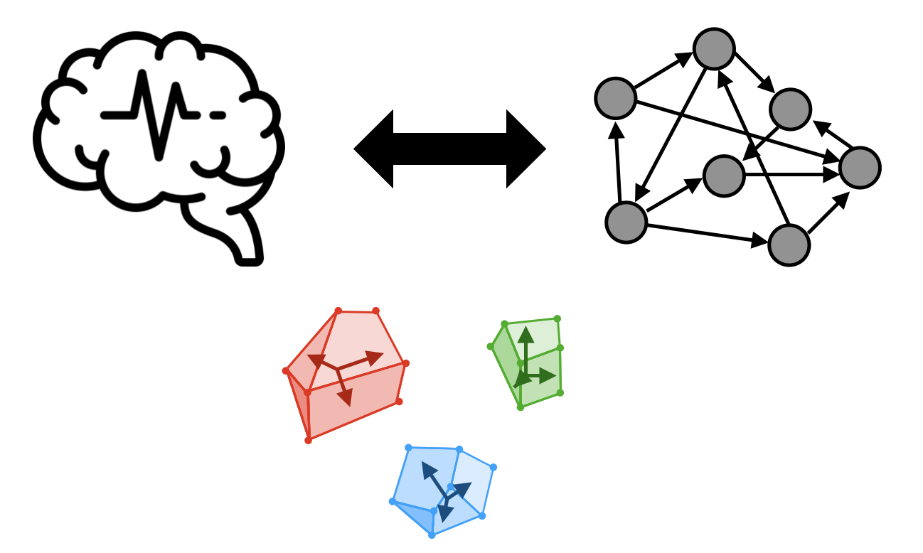
In recent years, growth in our understanding of the computations performed in both biological and artificial neural networks has largely been driven by either low-level mechanistic studies or global normative approaches. However, concrete methodologies for bridging the gap between these levels of abstraction remain elusive. In this work, we investigate the internal mechanisms of neural networks through the lens of neural population geometry, aiming to provide understanding at an intermediate level of abstraction, as a way to bridge that gap. Utilizing manifold capacity theory (MCT) from statistical physics and manifold alignment analysis (MAA) from high-dimensional statistics, we probe the underlying organization of task-dependent manifolds in deep neural networks and neural recordings from the macaque visual cortex. Specifically, we quantitatively characterize how different learning objectives lead to differences in the organizational strategies of these models and demonstrate how these geometric analyses are connected to the decodability of task-relevant information. Furthermore, these metrics show that macaque visual cortex data are more similar to unsupervised DNNs in terms of geometrical properties such as manifold position and manifold alignment. These analyses present a strong direction for bridging mechanistic and normative theories in neural networks through neural population geometry, potentially opening up many future research avenues in both machine learning and neuroscience.
Sensory cortex plasticity supports auditory social learning
Nihaad Paraouty, Justin D. Yao, Léo Varnet, Chi-Ning Chou, SueYeon Chung, Dan H. Sanes.
Nature Communications (2023).
[journal version][abstract ] [bibtex ]
@journal{paraouty2023sensory,
  title={Sensory cortex plasticity supports auditory social learning},
  author={Paraouty, Nihaad and Yao, Justin D and Varnet, L{\'e}o and Chou, Chi-Ning and Chung, SueYeon and Sanes, Dan H},
  journal={Nature Communications},
  volume={14},
  number={1},
  pages={5828},
  year={2023},
  publisher={Nature Publishing Group UK London}
}
Social learning (SL) through experience with conspecifics can facilitate the acquisition of many behaviors. Thus, when Mongolian gerbils are exposed to a demonstrator performing an auditory discrimination task, their subsequent task acquisition is facilitated, even in the absence of visual cues. Here, we show that transient inactivation of auditory cortex (AC) during exposure caused a significant delay in task acquisition during the subsequent practice phase, suggesting that AC activity is necessary for SL. Moreover, social exposure induced an improvement in AC neuron sensitivity to auditory task cues. The magnitude of neural change during exposure correlated with task acquisition during practice. In contrast, exposure to only auditory task cues led to poorer neurometric and behavioral outcomes. Finally, social information during exposure was encoded in the AC of observer animals. Together, our results suggest that auditory SL is supported by AC neuron plasticity occurring during social exposure and prior to behavioral performance.
Algorithmic Neuroscience
Neuroscience TCS Active
Can algorithmic thinking flourish our understanding in the brain? In this new research direction which I call “algorithmic neuroscience”, we want to study neuroscience by modeling systems and circuits as performing certain computation and trying to explore the underlying algorithmic ideas.
[Related papers ]ODE-Inspired Analysis for the Biological Version of Oja’s Rule in Solving Streaming PCA
with Mien Brabeeba Wang.
Conference on Learning Theory (COLT 2020).
[arxiv] [conference version (extended abstract)] [slides] [abstract ] [bibtex ]
@InProceedings{CW20,
  title = 	 {ODE-Inspired Analysis for the Biological Version of Oja{'}s Rule in Solving Streaming PCA},
  author = 	 {Chou, Chi-Ning and Wang, Mien Brabeeba},
  booktitle = 	 {Proceedings of Thirty Third Conference on Learning Theory (COLT 2020)},
  pages = 	 {1339--1343},
  year = 	 {2020},
  editor = 	 {Abernethy, Jacob and Agarwal, Shivani},
  volume = 	 {125},
  series = 	 {Proceedings of Machine Learning Research},
  month = 	 {09--12 Jul},
  publisher = 	 {PMLR},
  pdf = 	 {http://proceedings.mlr.press/v125/chou20a/chou20a.pdf},
  url = 	 {http://proceedings.mlr.press/v125/chou20a.html},
  archivePrefix = "arXiv",
  eprint = "1911.02363",
  primaryClass={q-bio.NC}
}
Oja's rule [Oja, Journal of mathematical biology 1982] is a well-known biologically-plausible algorithm using a Hebbian-type synaptic update rule to solve streaming principal component analysis (PCA). Computational neuroscientists have known that this biological version of Oja's rule converges to the top eigenvector of the covariance matrix of the input in the limit. However, prior to this work, it was open to prove any convergence rate guarantee.
In this work, we give the first convergence rate analysis for the biological version of Oja's rule in solving streaming PCA. Moreover, our convergence rate matches the information theoretical lower bound up to logarithmic factors and outperforms the state-of-the-art upper bound for streaming PCA. Furthermore, we develop a novel framework inspired by ordinary differential equations (ODE) to analyze general stochastic dynamics. The framework abandons the traditional step-by-step analysis and instead analyzes a stochastic dynamic in one-shot by giving a closed-form solution to the entire dynamic. The one-shot framework allows us to apply stopping time and martingale techniques to have a flexible and precise control on the dynamic. We believe that this general framework is powerful and should lead to effective yet simple analysis for a large class of problems with stochastic dynamics.
On the Algorithmic Power of Spiking Neural Networks
with Kai-Min Chung, Chi-Jen Lu.
Innovations in Theoretical Computer Science (ITCS 2019).
[arxiv] [conference version] [slides] [poster] [abstract ] [bibtex ]
@InProceedings{CCL19,
  author ={Chi-Ning Chou and Kai-Min Chung and Chi-Jen Lu},
  title ={On the Algorithmic Power of Spiking Neural Networks},
  booktitle ={10th Innovations in Theoretical Computer Science  Conference (ITCS 2019)},
  pages ={26:1--26:20},
  year ={2019},
  URL ={http://drops.dagstuhl.de/opus/volltexte/2018/10119},
  archivePrefix = "arXiv",
  eprint = "1803.10375",
  primaryClass={cs.NE}
}

Photo by Pennstatenews.
Spiking neural networks (SNNs) are mathematical models for biological neural networks such as our brain. In this work, we study SNNs through the lens of algorithms. In particular, we show that the firing rate of the integrate-and-fire SNN can efficiently solve the non-negative least squares problem and $\ell_1$ minimization problem. Further, our proof gives new interpretations on the integrate-and-fire SNN where the external charging and spiking effects can be viewed as gradient and projection respectively in the dual space.Quantum Advantage
Quantum Inactive
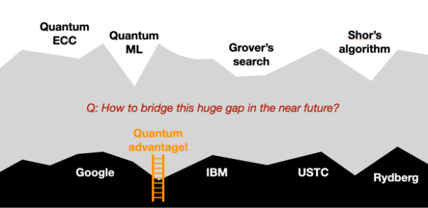
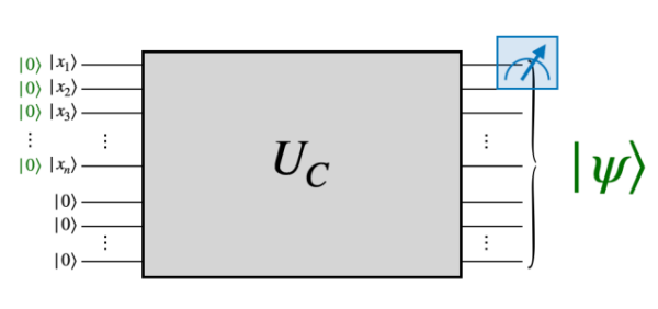
There is a huge gap between the theoretical endeavor and practical development of quantum computation. Quantum computational advantage is a bridge to propose near-term milestone to demonstrate the realizable computational power of quantum devices. I’m interested in both understanding better on the current quantum advantage proposals as well as proposing potentially useful quantum advantage tasks.
[Related papers ]Limitations of Linear Cross-Entropy as a Measure for Quantum Advantage
Xun Gao, Marcin Kalinowski, Chi-Ning Chou, Mikhail D. Lukin, Boaz Barak, Soonwon Choi.
Physical Review X Quantum (2024).
[journal version] [arxiv] [slides] [abstract ] [bibtex ]
@article{PRXQuantum.5.010334,
  title = {Limitations of Linear Cross-Entropy as a Measure for Quantum Advantage},
  author = {Gao, Xun and Kalinowski, Marcin and Chou, Chi-Ning and Lukin, Mikhail D. and Barak, Boaz and Choi, Soonwon},
  journal = {PRX Quantum},
  volume = {5},
  issue = {1},
  pages = {010334},
  numpages = {27},
  year = {2024},
  month = {Feb},
  publisher = {American Physical Society},
  doi = {10.1103/PRXQuantum.5.010334},
  url = {https://link.aps.org/doi/10.1103/PRXQuantum.5.010334}
}
Demonstrating quantum advantage requires experimental implementation of a computational task that is hard to achieve using state-of-the-art classical systems. One approach is to perform sampling from a probability distribution associated with a class of highly entangled many-body wavefunctions. It has been suggested that this approach can be certified with the Linear Cross-Entropy Benchmark (XEB). We critically examine this notion. First, in a "benign" setting where an honest implementation of noisy quantum circuits is assumed, we characterize the conditions under which the XEB approximates the fidelity. Second, in an "adversarial" setting where all possible classical algorithms are considered for comparison, we show that achieving relatively high XEB values does not imply faithful simulation of quantum dynamics. We present an efficient classical algorithm that, with 1 GPU within 2s, yields high XEB values, namely 2-12% of those obtained in experiments. By identifying and exploiting several vulnerabilities of the XEB, we achieve high XEB values without full simulation of quantum circuits. Remarkably, our algorithm features better scaling with the system size than noisy quantum devices for commonly studied random circuit ensembles. To quantitatively explain the success of our algorithm and the limitations of the XEB, we use a theoretical framework in which the average XEB and fidelity are mapped to statistical models. We illustrate the relation between the XEB and the fidelity for quantum circuits in various architectures, with different gate choices, and in the presence of noise. Our results show that XEB's utility as a proxy for fidelity hinges on several conditions, which must be checked in the benign setting but cannot be assumed in the adversarial setting. Thus, the XEB alone has limited utility as a benchmark for quantum advantage. We discuss ways to overcome these limitations.
Limitations of Local Quantum Algorithms on Maximum Cuts of Sparse Hypergraphs and Beyond
with Peter J. Love, Juspreet Singh Sandhu, Jonathan Shi.
International Colloquium on Automata, Languages and Programming (ICALP 2022).
[arxiv] [conference version] [abstract ] [bibtex ]
@InProceedings{CLSS22,
  author =	{Chou, Chi-Ning and Love, Peter J. and Sandhu, Juspreet Singh and Shi, Jonathan},
  title =	{Limitations of Local Quantum Algorithms on Random MAX-k-XOR and Beyond},
  booktitle =	{49th International Colloquium on Automata, Languages, and Programming (ICALP 2022)},
  pages =	{41:1--41:20},
  year =	{2022}
}
In this work, we study the limitations of the Quantum Approximate Optimization Algorithm (QAOA) through the lens of statistical physics and show that there exists $\epsilon > 0$, such that $\epsilon \log(n)$ depth QAOA cannot arbitrarily-well approximate the ground state energy of random diluted $k$-spin glasses when $k \geq 4$ is even. This is equivalent to the weak approximation resistance of logarithmic depth QAOA to the Max-$k$-XOR problem. We further extend the limitation to other boolean constraint satisfaction problems as long as the problem satisfies a combinatorial property called the coupled overlap-gap property (OGP) [Chen et al., Annals of Probability, 47(3), 2019]. As a consequence of our techniques, we confirm a conjecture of Brandao et al. [arXiv:1812.04170, 2018] asserting that the landscape independence of QAOA extends to logarithmic depth —-- in other words, for every fixed choice of QAOA angle parameters, the algorithm at logarithmic depth performs almost equally well on almost all instances. Our results provide a new way to study the power and limit of QAOA through statistical physics methods and combinatorial properties.
Spoofing Linear Cross-Entropy Benchmarking in Shallow Quantum Circuits
with Boaz Barak and Xun Gao.
Innovations in Theoretical Computer Science Conference (ITCS 2021).
[arxiv] [conference version] [slides] [abstract ] [bibtex ]
@InProceedings{BCG21,
  author =	{Boaz Barak and Chi-Ning Chou and Xun Gao},
  title =	{Spoofing Linear Cross-Entropy Benchmarking in Shallow Quantum Circuits},
  booktitle =	{12th Innovations in Theoretical Computer Science Conference (ITCS 2021)},
  pages =	{30:1--30:20},
  year =	{2021},
  archivePrefix = "arXiv",
  eprint = "2005.02421",
  primaryClass={quant-ph}
}
The linear cross-entropy benchmark (Linear XEB) has been used as a test for procedures simulating quantum circuits. Given a quantum circuit C with n inputs and outputs and purported simulator whose output is distributed according to a distribution p over $\{0,1\}^n$, the linear XEB fidelity of the simulator is $\mathcal{F}_C(p)=2^n\mathbb{E}_{x\sim p}q_C(x)-1$ where $q_C(x)$ is the probability that x is output from the distribution C|0n⟩. A trivial simulator (e.g., the uniform distribution) satisfies $\mathcal{F}_C(p)=0$, while Google's noisy quantum simulation of a 53 qubit circuit C achieved a fidelity value of (2.24±0.21)×10−3 (Arute et. al., Nature'19).
In this work we give a classical randomized algorithm that for a given circuit C of depth d with Haar random 2-qubit gates achieves in expectation a fidelity value of $\Omega(\frac{n}{L}\cdot15^{-d})$ in running time 𝗉𝗈𝗅𝗒(n,2L). Here L is the size of the *light cone* of C: the maximum number of input bits that each output bit depends on. In particular, we obtain a polynomial-time algorithm that achieves large fidelity of $\omega(1)$ for depth $O(\sqrt{\log n})$ two-dimensional circuits. To our knowledge, this is the first such result for two dimensional circuits of super-constant depth. Our results can be considered as an evidence that fooling the linear XEB test might be easier than achieving a full simulation of the quantum circuit.
Streaming Complexity
TCS Inactive
Streaming models are theoretical models for studying the scenario where input data is presented in a stream. We study the computational complexity of different problems with a focus on constraint satisfaction problems.
[Related papers ]Sketching Approximability of All Finite CSPs
with Alexander Golovnev, Madhu Sudan, Santhoshini Velusamy.
Journal of the ACM (2024).
[journal version] [arxiv] [abstract ] [bibtex ]
@journal{CGSV24J,
  author = {Chou, Chi-Ning and Golovnev, Alexander and Sudan, Madhu and Velusamy, Santhoshini},
  title = {Sketching Approximability of All Finite CSPs},
  year = {2024},
  publisher = {Association for Computing Machinery},
  address = {New York, NY, USA},
  issn = {0004-5411},
  url = {https://doi.org/10.1145/3649435},
  doi = {10.1145/3649435},
  journal = {J. ACM},
}
A constraint satisfaction problem (CSP), $\textsf{Max-CSP}(\mathcal{F})$, is specified by a finite set of constraints $\mathcal{F} \subseteq \{[q]^k \to \{0,1\}\}$ for positive integers $q$ and $k$. An instance of the problem on $n$ variables is given by $m$ applications of constraints from $\mathcal{F}$ to subsequences of the $n$ variables, and the goal is to find an assignment to the variables that satisfies the maximum number of constraints. In the $(\gamma,\beta)$-approximation version of the problem for parameters $0 \leq \beta < \gamma \leq 1$, the goal is to distinguish instances where at least $\gamma$ fraction of the constraints can be satisfied from instances where at most $\beta$ fraction of the constraints can be satisfied. In this work we consider the approximability of this problem in the context of sketching algorithms and give a dichotomy result. Specifically, for every family $\mathcal{F}$ and every $\beta < \gamma$, we show that either a linear sketching algorithm solves the problem in polylogarithmic space, or the problem is not solvable by any sketching algorithm in $o(\sqrt{n})$ space.
Linear Space Streaming Lower Bounds for Approximating CSPs
with Alexander Golovnev, Madhu Sudan, Ameya Velingker Santhoshini Velusamy.
Symposium on Theory of Computing (STOC 2022).
[arxiv] [eccc] [conference version] [abstract ] [bibtex ]
@article{CGSVV21,
  title={Linear Space Streaming Lower Bounds for Approximating CSPs},
  author={Chou, Chi-Ning and Golovnev, Alexander and Sudan, Madhu and Velingker, Ameya and Velusamy, Santhoshini},
  journal={arXiv preprint},
  year={2021},
  archivePrefix = "arXiv",
  eprint = "2106.13078",
  primaryClass={cs.CC}
}
We consider the approximability of constraint satisfaction problems in the streaming setting. For every constraint satisfaction problem (CSP) on n variables taking values in $\{0,\dots,q−1\}$, we prove that improving over the trivial approximability by a factor of $q$ requires $\Omega(n)$ space even on instances with $O(n)$ constraints. We also identify a broad subclass of problems for which any improvement over the trivial approximability requires $\Omega(n)$ space. The key technical core is an optimal, $q−(k−1)$-inapproximability for the case where every constraint is given by a system of $k−1$ linear equations mod $q$ over $k$ variables. Prior to our work, no such hardness was known for an approximation factor less than $1/2$ for any CSP. Our work builds on and extends the work of Kapralov and Krachun (Proc. STOC 2019) who showed a linear lower bound on any non-trivial approximation of the max cut in graphs. This corresponds roughly to the case of Max $k$-LIN-modq with $k=q=2$. Each one of the extensions provides non-trivial technical challenges that we overcome in this work.
Sketching Approximability of (Weak) Monarchy Predicates
with Alexander Golovnev, Amirbehshad Shahrasbi, Madhu Sudan, Santhoshini Velusamy.
Approximation, Randomization, and Combinatorial Optimization. Algorithms and Techniques (APPROX/RANDOM 2022).
[arxiv] [conference version] [abstract ] [bibtex ]
@article{CGSSV22,
  title={Sketching Approximability of (Weak) Monarchy Predicates},
  author={Chou, Chi-Ning and Golovnev, Alexander and Shahrasbi, Amirbehshad and Sudan, Madhu and Velusamy, Santhoshini},
  eprint={2205.02345},
  archivePrefix={arXiv},
  primaryClass={cs.CC}
}
We analyze the sketching approximability of constraint satisfaction problems on Boolean domains, where the constraints are balanced linear threshold functions applied to literals. In particular, we explore the approximability of monarchy-like functions where the value of the function is determined by a weighted combination of the vote of the first variable (the president) and the sum of the votes of all remaining variables. The pure version of this function is when the president can only be overruled by when all remaining variables agree. For every $k \geq 5$, we show that CSPs where the underlying predicate is a pure monarchy function on $k$ variables have no non-trivial sketching approximation algorithm in $o(\sqrt{n})$ space. We also show infinitely many weaker monarchy functions for which CSPs using such constraints are non-trivially approximable by $O(\log(n))$ space sketching algorithms. Moreover, we give the first example of sketching approximable asymmetric Boolean CSPs.
Our results work within the framework of Chou, Golovnev, Sudan, and Velusamy (FOCS 2021) that characterizes the sketching approximability of all CSPs. Their framework can be applied naturally to get a computer-aided analysis of the approximability of any specific constraint satisfaction problem. The novelty of our work is in using their work to get an analysis that applies to infinitely many problems simultaneously.
Approximability of all Finite CSPs with Linear Sketches
with Alexander Golovnev, Madhu Sudan, Santhoshini Velusamy.
Symposium on Foundations of Computer Science (FOCS 2021).
[arxiv] [eccc] [conference version] [slides] [abstract ] [bibtex ]
@article{CGSV21b,
  title={Approximability of all finite CSPs in the dynamic streaming setting},
  author={Chou, Chi-Ning and Golovnev, Alexander and Sudan, Madhu and Velusamy, Santhoshini},
  journal={arXiv preprint},
  year={2021},
  archivePrefix = "arXiv",
  eprint = "2105.01161",
  primaryClass={cs.CC}
}
A constraint satisfaction problem (CSP), Max-CSP($\mathcal{F}$), is specified by a finite set of constraints $\mathcal{F}\subseteq\{[q]^k\to\{0,1\}\}$ for positive integers $q$ and $k$. An instance of the problem on n variables is given by m applications of constraints from $\mathcal{F}$ to subsequences of the n variables, and the goal is to find an assignment to the variables that satisfies the maximum number of constraints. In the $(\gamma,\beta)$-approximation version of the problem for parameters $0\leq\beta\leq\gamma\leq1$, the goal is to distinguish instances where at least $\gamma$ fraction of the constraints can be satisfied from instances where at most $\beta$ fraction of the constraints can be satisfied.
In this work we consider the approximability of this problem in the context of sketching algorithms and give a dichotomy result. Specifically, for every family $\cF$ and every $\beta < \gamma$, we show that either a linear sketching algorithm solves the problem in polylogarithmic space, or the problem is not solvable by any sketching algorithm in $o(\sqrt{n})$ space.
Optimal Streaming Approximations for all Boolean Max 2-CSPs and Max k-SAT
with Alexander Golovnev, Santhoshini Velusamy.
Symposium on Foundations of Computer Science (FOCS 2020).
[arxiv] [conference version] [slides] [abstract ] [bibtex ]
@InProceedings{CGV20,
  title={Optimal Streaming Approximations for all Boolean Max-2CSPs and Max-ksat},
  author={Chou, Chi-Ning and Golovnev, Alexander and Velusamy, Santhoshini},
  booktitle={2020 IEEE 61st Annual Symposium on Foundations of Computer Science (FOCS)},
  year={2020},
  pages={330-341},
  doi={10.1109/FOCS46700.2020.00039},
  archivePrefix = "arXiv",
  eprint = "2004.11796",
  primaryClass={cs.CC}
}
We prove tight upper and lower bounds on approximation ratios of all Boolean Max-2CSP problems in the streaming model. Specifically, for every type of Max-2CSP problem, we give an explicit constant $\alpha$, s.t. for any $\epsilon>0$ (i) there is an $(\alpha-\epsilon)$-streaming approximation using space $O(\log n)$; and (ii) any $(\alpha-\epsilon)$-streaming approximation requires space $\Omega(\sqrt{n})$. This generalizes the celebrated work of [Kapralov, Khanna, Sudan SODA 2015; Kapralov, Krachun STOC 2019], who showed that the optimal approximation ratio for Max-CUT was 1/2.
Prior to this work, the problem of determining this ratio was open for all other Max-2CSPs. Our results are quite surprising for some specific Max-2CSPs. For the Max-DCUT problem, there was a gap between an upper bound of 1/2 and a lower bound of 2/5 [Guruswami, Velingker, Velusamy APPROX 2017]. We show that neither of these bounds is tight, and the optimal ratio for Max-DCUT is 4/9. We also establish that the tight approximation for Max-2SAT is $\sqrt{2}/2$, and for Exact Max-2SAT it is 3/4. As a byproduct, our result gives a separation between space-efficient approximations for Max-2SAT and Exact Max-2SAT. This is in sharp contrast to the setting of polynomial-time algorithms with polynomial space, where the two problems are known to be equally hard to approximate.
Tracking the $\ell_2$ Norm with Constant Update Time
with Zhixian Lei, Preetum Nakkiran.
Approximation, Randomization, and Combinatorial Optimization. Algorithms and Techniques (APPROX/RANDOM 2019).
[arxiv] [conference version] [slides] [abstract ] [bibtex ]
@InProceedings{CLN19,
  author =	{Chi-Ning Chou and Zhixian Lei and Preetum Nakkiran},
  title =	{Tracking the l_2 Norm with Constant Update Time},
  booktitle =	{Approximation, Randomization, and Combinatorial Optimization. Algorithms and Techniques (APPROX/RANDOM 2019)},
  pages =	{2:1--2:15},
  ISSN =	{1868-8969},
  year =	{2019},
  URL =		{http://drops.dagstuhl.de/opus/volltexte/2019/11217},
  URN =		{urn:nbn:de:0030-drops-112175},
  annote =	{Keywords: Streaming algorithms, Sketching algorithms, Tracking, CountSketch},
  archivePrefix = "arXiv",
  eprint = "1807.06479",
  primaryClass={cs.DS}
}
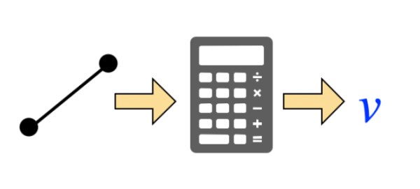
The $\ell_2$ tracking problem is the task of obtaining a streaming algorithm that, given access to a stream of items $a_1,a_2,a_3,\ldots$ from a universe $[n]$, outputs at each time $t$ an estimate to the $\ell_2$ norm of the frequency vector $f^{(t)}\in \mathbb{R}^n$ (where $f^{(t)}_i$ is the number of occurrences of item $i$ in the stream up to time $t$). The previous work [Braverman-Chestnut-Ivkin-Nelson-Wang-Woodruff, PODS 2017] gave an streaming algorithm with (the optimal) space using $O(\epsilon^{-2}\log(1/\delta))$ words and $O(\epsilon^{-2}\log(1/\delta))$ update time to obtain an $\epsilon$-accurate estimate with probability at least $1-\delta$.
We give the first algorithm that achieves update time of $O(\log 1/\delta)$ which is independent of the accuracy parameter $\epsilon$, together with the nearly optimal space using $O(\epsilon^{-2}\log(1/\delta))$ words. Our algorithm is obtained using the Count Sketch of [Charilkar-Chen-Farach-Colton, ICALP 2002].
Quantum Complexity
Quantum TCS Inactive
Complexity theory studies the quantitative relation between different resources (e.g., time, space, entanglement, circuit size, number of samples). I’m interested in studying various quantum systems through complexity-theoretic lens and reveal new physical insights.
[Related papers ]Quantum Meets the Minimum Circuit Size Problem
with Nai-Hui Chia, Jiayu Zhang, Ruizhe Zhang.
Innovations in Theoretical Computer Science Conference (ITCS 2022).
[arxiv] [eccc] [conference version] [slides] [abstract ] [bibtex ]
@inproceedings{CCZZ21,
  title={Quantum Meets the Minimum Circuit Size Problem},
  author={Chia, Nai-Hui and Chou, Chi-Ning and Zhang, Jiayu and Zhang, Ruizhe},
  booktitle={13th Innovations in Theoretical Computer Science Conference (ITCS 2022)},
  year={2022}
}
In this work, we initiate the study of the Minimum Circuit Size Problem (MCSP) in the quantum setting. MCSP is a problem to compute the circuit complexity of Boolean functions. It is a fascinating problem in complexity theory---its hardness is mysterious, and a better understanding of its hardness can have surprising implications to many fields in computer science.
We first define and investigate the basic complexity-theoretic properties of minimum quantum circuit size problems for three natural objects: Boolean functions, unitaries, and quantum states. We show that these problems are not trivially in NP but in QCMA (or have QCMA protocols). Next, we explore the relations between the three quantum MCSPs and their variants. We discover that some reductions that are not known for classical MCSP exist for quantum MCSPs for unitaries and states, e.g., search-to-decision reduction and self-reduction. Finally, we systematically generalize results known for classical MCSP to the quantum setting (including quantum cryptography, quantum learning theory, quantum circuit lower bounds, and quantum fine-grained complexity) and also find new connections to tomography and quantum gravity. Due to the fundamental differences between classical and quantum circuits, most of our results require extra care and reveal properties and phenomena unique to the quantum setting. Our findings could be of interest for future studies, and we post several open problems for further exploration along this direction.
Spiking Neural Networks
Neuroscience Inactive
One of the main differences between biological neural networks and artificial neural networks (ANNs) is the way neurons interact with each other: while the former use instantaneous spikes, the latter use continuous (digital) signals. The main research questions I’m exploring are what’s the fundamental differences between spiking neural networks (SNNs) and ANNs and what are the different roles of spikes can play in the brain. On the practical side, I’m also very interested in demonstrating spiking computational advantage, e.g., through neuromorphic computing.
[Related papers ]A Superconducting Nanowire-based Architecture for Neuromorphic Computing
Andres E. Lombo, Jesus E. Lares, Matteo Castellani, Chi-Ning Chou, Nancy Lynch, Karl K. Berggren.
Neuromorphic Computing and Engineering (2022).
NCE Highlights of 2022.
[journal version] [arxiv] [abstract ] [bibtex ]
@article{LLCCLB22,
  title={A Superconducting Nanowire-based Architecture for Neuromorphic Computing},
  author={Lombo, Andres E. and Lares, Jesus E. and Castellani, Matteo and Chou, Chi-Ning and Lynch, Nancy and Berggren, Karl K.},
  journal={Neuromorphic Computing and Engineering},
  year={2022},
  publisher={IOP Publishing},
  url={http://iopscience.iop.org/article/10.1088/2634-4386/ac86ef}
}
Neuromorphic computing is poised to further the success of software-based neural networks by utilizing improved customized hardware. However, the translation of neuromorphic algorithms to hardware specifications is a problem that has been seldom explored. Building superconducting neuromorphic systems requires extensive expertise in both superconducting physics and theoretical neuroscience. In this work, we aim to bridge this gap by presenting a tool and methodology to translate algorithmic parameters into circuit specifications. We first show the correspondence between theoretical neuroscience models and the dynamics of our circuit topologies. We then apply this tool to solve linear systems by implementing a spiking neural network with our superconducting nanowire-based hardware.
On the Algorithmic Power of Spiking Neural Networks
with Kai-Min Chung, Chi-Jen Lu.
Innovations in Theoretical Computer Science (ITCS 2019).
[arxiv] [conference version] [slides] [poster] [abstract ] [bibtex ]
@InProceedings{CCL19,
  author ={Chi-Ning Chou and Kai-Min Chung and Chi-Jen Lu},
  title ={On the Algorithmic Power of Spiking Neural Networks},
  booktitle ={10th Innovations in Theoretical Computer Science  Conference (ITCS 2019)},
  pages ={26:1--26:20},
  year ={2019},
  URL ={http://drops.dagstuhl.de/opus/volltexte/2018/10119},
  archivePrefix = "arXiv",
  eprint = "1803.10375",
  primaryClass={cs.NE}
}
Photo by Pennstatenews.
Spiking neural networks (SNNs) are mathematical models for biological neural networks such as our brain. In this work, we study SNNs through the lens of algorithms. In particular, we show that the firing rate of the integrate-and-fire SNN can efficiently solve the non-negative least squares problem and $\ell_1$ minimization problem. Further, our proof gives new interpretations on the integrate-and-fire SNN where the external charging and spiking effects can be viewed as gradient and projection respectively in the dual space.Circuit Complexity
TCS Inactive
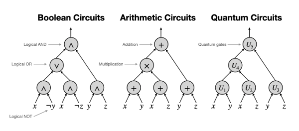
Circuits are one of the fundamental computational models in the theory of computation. I’m interested in various circuit models (e.g., boolean circuits, arithmetic circuits, quantum circuits, and their special variants)and study the relation between circuit complexity and other aspects of computational problems.
[Related papers ]Closure Results for Polynomial Factorization
with Mrinal Kumar, Noam Solomon.
Theory of Computing (2019).
[journal version] [slides] [video] [abstract ] [bibtex ]
@journal{CKS19J,
  author = {Chou, Chi-Ning and Kumar, Mrinal and Solomon, Noam},
  title = {Closure Results for Polynomial Factorization},
  year = {2019},
  pages = {1--34},
  doi = {10.4086/toc.2019.v015a013},
  publisher = {Theory of Computing},
  journal = {Theory of Computing},
  volume = {15},
  number = {13},
  URL = {http://www.theoryofcomputing.org/articles/v015a013},
  archivePrefix = "arXiv",
  eprint = "1803.05933",
  primaryClass={cs.CC}
}
In a sequence of fundamental results in the 1980s, Kaltofen (SICOMP 1985, STOC'86, STOC'87, RANDOM'89) showed that factors of multivariate polynomials with small arithmetic circuits have small arithmetic circuits. In other words, the complexity class $\VP$ is closed under taking factors. A natural question in this context is to understand if other natural classes of multivariate polynomials, for instance, arithmetic formulas, algebraic branching programs, bounded-depth arithmetic circuits or the class $\VNP$, are closed under taking factors.
In this paper, we show that all factors of degree $\log^a n$ of polynomials with $\poly(n)$-size depth-$k$ circuits have $\poly(n)$-size circuits of depth $O(k + a)$. This partially answers a question of Shpilka--Yehudayoff (Found. Trends in TCS, 2010) and has applications to hardness-randomness tradeoffs for bounded-depth arithmetic circuits.
As direct applications of our techniques, we also obtain simple proofs of the following results.
$\bullet$ The complexity class $\VNP$ is closed under taking factors. This confirms Conjecture~2.1 in Bürgisser's monograph (2000) and improves upon a recent result of Dutta, Saxena and Sinhababu (STOC'18) who showed a quasipolynomial upper bound on the number of auxiliary variables and the complexity of the verifier circuit of factors of polynomials in $\VNP$.
$\bullet$ A factor of degree $d$ of a polynomial $P$ which can be computed by an arithmetic formula (or an algebraic branching program) of size $s$ has a formula (an algebraic branching program, resp.) of size $\poly(s, d^{\log d}, \deg(P))$. This result was first shown by Dutta et al. (STOC'18) and we obtain a slightly different proof as an easy consequence of our techniques.
Our proofs rely on a combination of the ideas, based on Hensel lifting, developed in the polynomial factoring literature, and the depth-reduction results for arithmetic circuits, and hold over fields of characteristic zero or of sufficiently large characteristic.
Closure of $\VP$ under taking factors: a short and simple proof
with Mrinal Kumar, Noam Solomon.
Manuscript.
[arxiv] [eccc] [abstract ] [bibtex ]
@unpublished{CKS19,
  title={Closure of VP under taking factors: a short and simple proof},
  author={Chou, Chi-Ning and Kumar, Mrinal and Solomon, Noam},
  note={In submission to Theory of Computing},
  eprint={1903.02366},
  archivePrefix={arXiv},
  primaryClass={cs.CC}
}
In this note, we give a short, simple and almost completely self contained proof of a classical result of Kaltofen which shows that if an $n$ variate degree $d$ polynomial $f$ can be computed by an arithmetic circuit of size $s$, then each of its factors can be computed by an arithmetic circuit of size at most $\poly\left(s, n, d\right)$.
However, unlike Kaltofen's argument, our proof does not directly give an efficient algorithm for computing the circuits for the factors of $f$.
Hardness vs Randomness for Bounded Depth Arithmetic Circuits
with Mrinal Kumar, Noam Solomon.
Computational Complexity Conference (CCC 2018).
[arxiv] [eccc] [conference version] [slides] [abstract ] [bibtex ]
@InProceedings{CKS18,
  author ={Chi-Ning Chou and Mrinal Kumar and Noam Solomon},
  title ={Hardness vs Randomness for Bounded Depth Arithmetic Circuits},
  booktitle ={33rd Computational Complexity Conference (CCC 2018)},
  pages ={13:1--13:17},
  ISSN ={1868-8969},
  year ={2018},
  URL ={http://drops.dagstuhl.de/opus/volltexte/2018/8876},
  URN ={urn:nbn:de:0030-drops-88765},
  annote ={Keywords: Algebraic Complexity, Polynomial Factorization Circuit Lower Bounds, Polynomial Identity Testing}
}
In this paper, we study the question of hardness-randomness tradeoffs for bounded depth arithmetic circuits. We show that if there is a family of explicit polynomials $\{f_n\}$, where $f_n$ is of degree $O(\log^2n/\log^2\log n)$ in $n$ variables such that $f_n$ cannot be computed by a depth $\Delta$ arithmetic circuits of size $\poly(n)$, then there is a deterministic sub-exponential time algorithm for polynomial identity testing of arithmetic circuits of depth $\Delta-5$.
This is incomparable to a beautiful result of Dvir et al.[SICOMP, 2009], where they showed that super-polynomial lower bounds for depth $\Delta$ circuits for any explicit family of polynomials (of potentially high degree) implies sub-exponential time deterministic PIT for depth $\Delta-5$ circuits of bounded individual degree. Thus, we remove the ``bounded individual degree" condition in the work of Dvir et al. at the cost of strengthening the hardness assumption to hold for polynomials of low degree.
The key technical ingredient of our proof is the following property of roots of polynomials computable by a bounded depth arithmetic circuit : if $f(x_1, x_2, \ldots, x_n)$ and $P(x_1, x_2, \ldots, x_n, y)$ are polynomials of degree $d$ and $r$ respectively, such that $P$ can be computed by a circuit of size $s$ and depth $\Delta$ and $P(x_1, x_2, \ldots, x_n, f) \equiv 0$, then, $f$ can be computed by a circuit of size $\poly(n, s, r, d^{O(\sqrt{d})})$ and depth $\Delta + 3$. In comparison, Dvir et al. showed that $f$ can be computed by a circuit of depth $\Delta + 3$ and size $\poly(n, s, r, d^{t})$, where $t$ is the degree of $P$ in $y$. Thus, the size upper bound in the work of Dvir et al. is non-trivial when $t$ is small but $d$ could be large, whereas our size upper bound is non-trivial when $d$ is small, but $t$ could be large.